Eigenpairs from Matrix–Vector Products: Power Iteration, Deflation, Lanczos, and Arnoldi
Linear AlgebraEigenvaluesPower IterationLanczos MethodArnoldi MethodMatrix-Free Methods
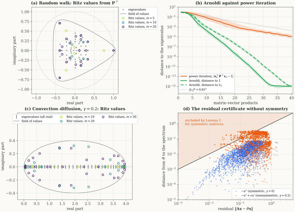
This document rigorously studies what can be learned about the A nonzero vector u is an eigenvector of A, with eigenvalueλ, when Au=λu. Multiplying u by A only rescales it, by the factor λ, and the pair (λ,u) is called an eigenpair. For example, A=[2112] maps [1,1]⊤ to 3[1,1]⊤ and [1,−1]⊤ to itself, so these two vectors are eigenvectors, with the eigenvalues 3 and 1. Rewriting the definition as (A−λId)u=0 shows that λ is an eigenvalue exactly when the matrix A−λId is singular, that is, when λ is a root of the polynomial λ↦det(λId−A), of degree d, called the characteristic polynomial of A. The eigenvectors of λ are then the nonzero vectors of the null space ker(A−λId), called the eigenspace of λ. A real polynomial can have complex roots, so a real matrix can have complex eigenvalues. The rotation [01−10] turns every real vector by a quarter turn, so it has no real eigenvector, and its characteristic polynomial λ2+1 has the roots ±i. A real symmetric matrix, in contrast, has only real eigenvalues and an orthonormal basis of eigenvectors, by the spectral theorem used in Sections 1 to 4. Computing the characteristic polynomial requires every entry of A, which the setting of this post does not provide. The definition itself, however, involves A only through the product Au. One product is enough to test a candidate pair (λ,u), because the residual Au−λu=(A−λId)u vanishes exactly when the pair is an eigenpair. The methods of this post use A in no other way. For a symmetric matrix, Lemma 2 and Remark 11 also turn a small residual into a guarantee: if ∥u∥=1, then λ is within ∥Au−λu∥ of an eigenvalue. of a real matrix A∈Rd×d that is known only through the map x↦Ax. Storing A takes d2 numbers, and forming it can cost much more. In many applications, however, the product Ax is cheap, because it follows directly from how A is defined, whether A is built from a data matrix, a sparse graph or a discretized differential operator, or is the Hessian of a function whose gradient can be computed (Section 2 gives more examples). Two families of methods need nothing more than such products: power iteration (Section 3), which extracts one eigenpair at a time and reaches further eigenpairs through shifts and deflation, and the Lanczos method (Section 4), which builds an orthonormal basis of a Krylov subspace and solves a small tridiagonal eigenvalue problem inside it. Sections 1 to 4 assume that A is symmetric, as Hessians, covariance matrices and the adjacency matrices of undirected graphs are. The Arnoldi method (Section 5) extends the Lanczos method to nonsymmetric matrices, such as the transition matrix of a random walk on a directed graph.
The results assume neither positive definiteness nor distinct eigenvalues. Each statement says precisely which eigenpairs are recovered, and the remarks say which are not. All the delicate cases are treated explicitly: a dominant eigenvalue of either sign, opposite eigenvalues of equal magnitude, repeated eigenvalues, and zero eigenvalues. Sections 3, 4 and 5 each end with an implementable procedure: Algorithm 1 for power iteration, Algorithm 2 for the Lanczos method and Algorithm 3 for the Arnoldi method. All three stop when a residual computed with the original matrix falls below a tolerance. The figures run these procedures on matrices with prescribed spectra and on five matrices from applications: the adjacency matrix of a graph, a covariance matrix and the Hessian of a neural network (Section 2), and the transition matrix of a random walk on a directed graph and a discretized convection–diffusion operator (Section 5.1). The code that produces them, with implementations of the three algorithms, is on GitHub.
For a symmetric A, the central object is the decomposition of a vector along the eigenspaces of A. Let Λ(A) be the set of distinct eigenvalues of A, and let Πλ be the orthogonal projection onto the eigenspace of λ∈Λ(A). Then, for every vector v∈Rd and every integer k≥0,
v=λ∈Λ(A)∑Πλv,Akv=λ∈Λ(A)∑λkΠλv.
Started from v, power iteration keeps the last vector of the sequence v,Av,A2v,… and lets the factors λk select the eigenvalue of largest magnitude. The Lanczos method keeps the whole sequence and optimizes over its span. Every proof of Sections 3 and 4 follows the components Πλv through these operations, and Section 5 shows what changes when the eigenspaces are no longer orthogonal.
1. Notation and preliminaries
Notation
∥⋅∥ is the Euclidean norm, Id the d×d identity matrix, δiℓ the Kronecker delta, and em=[0,…,0,1]⊤∈Rm the last standard basis vector of Rm.
For a subspace S⊆Rd, S⊥={x∈Rd:x⊤s=0∀s∈S} is its orthogonal complement.
For a matrix M with n columns, ker(M)={x∈Rn:Mx=0} is its null space and range(M)={Mx:x∈Rn} is its column space.
In Sections 1 to 4, A∈Rd×d is symmetric, and Section 5 drops this assumption. We let Λ(A) be the set of its distinct eigenvalues, so that a repeated eigenvalue appears once in Λ(A), and we write λmin(A)=minΛ(A) and λmax(A)=maxΛ(A).
For each λ∈Λ(A), Eλ=ker(A−λId) is the eigenspace of λ, and Πλ is the orthogonal projection onto Eλ. If the columns u1,…,umλ of Uλ∈Rd×mλ form an orthonormal basis of Eλ, where mλ is the multiplicity of λ, then Πλ=UλUλ⊤=∑i=1mλuiui⊤, that is, Πλx=∑i=1mλ(ui⊤x)ui keeps the components of x along these basis vectors. An expression in terms of A alone is given below.
For vectors u1,…,um∈Rd, [u1,…,um]∈Rd×m is the matrix with these columns, and span{u1,…,um} is the set of their linear combinations
diag(c1,…,cm) is the diagonal matrix with diagonal entries c1,…,cm∈R.
N(0,Id) is the standard Gaussian distribution on Rd, and sgn(t)∈{−1,1} is the sign of a real number t=0.
Spectral decomposition
When A is symmetric, the Every real symmetric matrix has an orthonormal basis of eigenvectors. Collecting the basis vectors that share the eigenvalue λ as the columns of a matrix Uλ gives Πλ=UλUλ⊤, and the three identities follow from the orthonormality of the basis. gives
A=λ∈Λ(A)∑λΠλ,Id=λ∈Λ(A)∑Πλ,ΠλΠμ=0when λ=μ.
The powers of A act on each eigenspace separately, and so does every polynomial:
for every integer k≥0 and every polynomial p,
Ak=λ∈Λ(A)∑λkΠλ,p(A)=λ∈Λ(A)∑p(λ)Πλ.
In fact, each column ui of Uλ is an eigenvector, Aui=λui, so multiplying Πλ=∑i=1mλuiui⊤ by A gives AΠλ=∑i=1mλ(Aui)ui⊤=λΠλ.
The spectral theorem gives the same identity, since AΠλ=∑μμΠμΠλ=λΠλ2 and Πλ2=Πλ. Applying it k times gives AkΠλ=λkΠλ, and multiplying Id=∑λΠλ by Ak then gives the first identity above.
For a polynomial p(t)=∑k=0ncktk, we have p(A)=∑k=0nckAk=∑λ(∑k=0nckλk)Πλ=∑λp(λ)Πλ, which is the second identity.
Taking for p the Given finitely many distinct numbers, the Lagrange polynomial attached to one of them equals 1 at that number and 0 at all the others. For λ∈Λ(A) it is ℓλ(t)=μ∈Λ(A),μ=λ∏λ−μt−μ. Each factor vanishes at its own μ and equals 1 at t=λ, so ℓλ(λ)=1 and ℓλ(μ)=0 for every other μ∈Λ(A). Its degree is ∣Λ(A)∣−1. Substituting it for p in p(A)=∑νp(ν)Πν keeps only the term ν=λ, so ℓλ(A)=Πλ. For example, if Λ(A)={1,3}, then ℓ1(t)=(3−t)/2 and Π1=(3Id−A)/2. that equals 1 at λ and 0 at the other distinct eigenvalues expresses each projection through A alone:
Πλ=μ∈Λ(A)μ=λ∏λ−μA−μId,
where the empty product, when A has a single distinct eigenvalue, equals Id.
These projections are used in the analysis. The algorithms below do not require computing them.
2. Matrices known only through their products
The results below use A only through the products x↦Ax, so they hold whatever routine computes those products. The following cases are typical.
2.1 Hessians
In many problems, A=∇θ2f(θ) is the Hessian of a function f:Rd→R that is twice continuously differentiable in a neighborhood of a point θ. Examples include the following.
Training losses. The training loss of a (deep) neural network with parameters θ is f(θ)=n1∑i=1nℓ(zi(θ),yi), where zi(θ) is the output of the network on the i-th of n training inputs, yi is the target for that input, and ℓ is a cost function such as ℓ(z,y)=21∥z−y∥2. Its curvature is studied to understand optimization (how training progresses) and generalization (how the network performs on new inputs).
Likelihoods. The negative log-likelihood of observations y1,…,yn under a statistical model with density p(⋅;θ) is f(θ)=−∑i=1nlogp(yi;θ). Its minimizer θ^ is the maximum-likelihood estimate, and the Hessian ∇2f(θ^) is the observed Fisher information. For large samples, its inverse approximates the covariance of θ^, that is, how precisely the data determine the parameters.
Newton-type optimization. To minimize f(θ), Near θ, Newton’s method replaces f by its second-order Taylor expansion, a quadratic function of the step: f(θ+Δθ)≈f(θ)+∇f(θ)⊤Δθ+21Δθ⊤∇2f(θ)Δθ. The gradient of this model with respect to Δθ is ∇f(θ)+∇2f(θ)Δθ, and setting it to zero gives the linear system ∇2f(θ)Δθ=−∇f(θ). When ∇2f(θ) is positive definite, the model is a bowl and Δθ goes to its bottom. Otherwise, the model has no minimum, and practical methods modify the step. In one dimension, the step Δθ=−f′(θ)/f′′(θ) moves to the point where the tangent line of f′ at θ crosses zero, as Newton’s method does to solve f′=0. Write the Hessian in an orthonormal eigenbasis, ∇2f(θ)=∑j=1dλjujuj⊤, with every λj>0. Since ui⊤uj=δij, multiplying the sum on the left by ui⊤ gives ui⊤∇2f(θ)=λiui⊤. Multiplying the linear system on the left by ui⊤ therefore gives λiui⊤Δθ=−ui⊤∇f(θ), that is, ui⊤Δθ=−ui⊤∇f(θ)/λi. Expanding the step in the same basis, Δθ=∑i=1d(ui⊤Δθ)ui, and substituting each coordinate gives Δθ=−i=1∑dλiui⊤∇f(θ)ui. Each component of the gradient is divided by the curvature λi along ui, so the step is short where f is steep and long where f is flat. Gradient descent instead takes the step Δθ=−α∇f(θ)=−i=1∑dα(ui⊤∇f(θ))ui, which multiplies every coordinate by the same factor α. takes the step Δθ that solves the linear system ∇2f(θ)Δθ=−∇f(θ). Solving it by forming and factorizing the d×d Hessian would take d2 numbers of storage and about d3 operations. Truncated Newton methods (Dembo and Steihaug, 1983) instead run a few iterations of the conjugate gradient method (Hestenes and Stiefel, 1952), which uses the Hessian only through products ∇2f(θ)x, computed as explained below, and stop once the step is accurate enough. The conjugate gradient method builds the same Krylov subspaces as the Lanczos method.
Molecular vibrations. The potential energy f(θ) of a molecule depends on the positions θ∈R3N of its N atoms. Near an equilibrium θ⋆, where ∇f(θ⋆)=0, small displacements obey Newton’s second law says that mass times acceleration equals force, and the force on the atoms is minus the gradient of the potential energy, −∇f(θ): the atoms are pushed downhill. Near θ⋆, the first-order Taylor expansion of the gradient is ∇f(θ)≈∇f(θ⋆)+∇2f(θ⋆)(θ−θ⋆)=∇2f(θ⋆)(θ−θ⋆), because ∇f(θ⋆)=0 at an equilibrium. The force is therefore a linear restoring force, as for a system of springs, and Mθ¨=−∇f(θ) becomes the stated equation, where θ¨ is the acceleration, the second time derivative of the positions.Mθ¨=−∇2f(θ⋆)(θ−θ⋆), where M is the diagonal matrix of atomic masses, each repeated for the three coordinates of its atom. The eigenvectors of the In the mass-weighted coordinates x=M1/2(θ−θ⋆), substituting θ−θ⋆=M−1/2x into the equation of motion and multiplying it on the left by M−1/2 gives x¨=−Kx,K=M−1/2∇2f(θ⋆)M−1/2. A motion in which every coordinate oscillates at the same frequency ω in a fixed pattern v, x(t)=cos(ωt)v, has x¨=−ω2x, so it solves the equation exactly when Kv=ω2v. Each eigenvector of K is thus a vibration pattern, a normal mode, and its eigenvalue is the squared frequency of that mode. Because K is symmetric, its orthonormal eigenvectors split every small motion into independent normal modes, each vibrating at its own frequency, and the weighting by M−1/2 on both sides is what keeps the matrix symmetric. At a minimum of f, the Hessian is positive semidefinite, and so is K, since x⊤Kx=(M−1/2x)⊤∇2f(θ⋆)(M−1/2x)≥0. Its eigenvalues are therefore nonnegative, and each one is the square of a real frequency ω. At a saddle point of f, an eigenvalue −μ<0 would have no real square root, and the displacement along its mode would grow like eμt instead of oscillating. For example, take two atoms of masses m1 and m2 at positions θ1 and θ2 on a line, joined by a spring of stiffness k and rest length a. The energy of the spring is f(θ)=2k(θ2−θ1−a)2, and ∇2f(θ⋆)=k[1−1−11],K=k[1/m1−1/m1m2−1/m1m21/m2]. The eigenvalues of K are 0, whose mode moves both atoms together and stretches nothing, and k(1/m1+1/m2), the trace of K. The second mode moves the atoms in opposite directions, the heavier one less, and it is the stretching vibration, with frequency ω=k(1/m1+1/m2).M−1/2∇2f(θ⋆)M−1/2 are the vibration patterns of the molecule (its normal modes), and its eigenvalues are the squared vibration frequencies ω2. A product with this matrix is a Hessian–vector product between two diagonal scalings, M−1/2(∇2f(θ⋆)(M−1/2x)), so the lowest-frequency modes of a large molecule, its slowest collective motions, can be computed without forming the 3N×3N Hessian.
Such a Hessian is symmetric by When the second partial derivatives of f are continuous near θ, they do not depend on the order of differentiation: ∂2f/∂θi∂θj=∂2f/∂θj∂θi. The Hessian is therefore a real symmetric matrix.. In that case, each product can be evaluated as
Ax=∇θ(∇θf(θ)⊤x),
with x held constant during differentiation. The scalar ∇θf(θ)⊤x is the directional derivative of f along x. Its gradient with respect to θ is ∇θ2f(θ)⊤x, which equals Ax because the Hessian is symmetric. Automatic differentiation therefore returns the product at a The product is obtained by differentiating the gradient computation once more, in forward or reverse mode. Each pass costs a small constant multiple of the original computation, so the product costs about as much as a few gradient evaluations. (Pearlmutter, 1994), and the d×d matrix is never formed.
The point θ and everything that defines f must remain fixed during an eigensolver run. For a training loss, evaluating it on a different random subset of the data (a minibatch) between two products changes the matrix being analyzed, and the statements below then no longer describe the computation.
Every symmetric matrix A is in fact a Hessian: the quadratic x↦21x⊤Ax has the Hessian A at every point. This does not help to compute products, since the gradient of that quadratic is Ax itself. The Hessian route pays off when f is given by a program whose gradient is cheap, so that curvature is obtained from first-order code. For the matrices of the following section, the products come instead from the structure that defines A.
2.2 Other matrices known through their products
Products are just as cheap in many cases where A is not presented as a Hessian.
Gram and covariance matrices. For a data matrix X∈Rn×d, whose n rows are observations of d variables, the product X⊤Xx=X⊤(Xx)The parentheses fix the order: two matrix–vector products, and X⊤X is never formed. First, each of the n entries of y=Xx is the inner product of a row of X with x, about d multiplications and additions. Then each of the d entries of X⊤y is the inner product of a column of X with y, about n of them. Each pass costs about nd operations, and only y is stored in between. Forming X⊤X instead takes d2 inner products of columns of length n, about nd2 operations, and d2 numbers of storage. For n=106 observations of d=104 variables, one product costs about 2⋅1010 operations, whereas forming X⊤X costs about 1014 operations and 108 numbers of storage. If X is sparse, a product costs on the order of its number of nonzero entries., whereas forming X⊤X costs O(nd2) and storing it costs O(d2). When each column of X has zero mean, the sample covariance matrix of the d variables is the average of the outer products of the observations, X⊤X/n=(1/n)∑i=1nXiXi⊤, where Xi∈Rd is the i-th row of X. Its leading eigenvector, the first principal component, is the direction of largest variance in the data: it maximizes the variance n1∥Xu∥2 of the data projected on u over unit vectors u.
Gauss–Newton matrices. Many objectives are compositions f(θ)=ψ(F(θ)) of a map F:Rd→Rp and a function ψ:Rp→R, both twice differentiable. For the training loss of Section 2.1, F(θ) stacks the outputs z1(θ),…,zn(θ) into one vector of Rp, and ψ(z)=n1∑i=1nℓ(zi,yi) for z=[z1;…;zn]. Let J∈Rp×d be the Jacobian of F at θ, with entries Jkj=∂Fk(θ)/∂θj, and let H=∇2ψ(F(θ))∈Rp×p. The chain rule gives ∇2f(θ)=J⊤HJ+∑k=1p∂kψ(F(θ))∇2Fk(θ), where ∂kψ is the partial derivative of ψ with respect to its k-th argument. The generalized Gauss–Newton matrix G=J⊤HJ keeps the first term. It is symmetric, and positive semidefinite when ψ is convex. It is applied as Gx=J⊤(H(Jx)), where automatic differentiation computes Jx in forward mode and J⊤u in reverse mode without forming J. For least squares, ψ(z)=21∥z−y∥2 for a target y∈Rp, so H=Ip and G=J⊤J. When F is linear, F(θ)=Jθ, every ∇2Fk vanishes and G is the exact Hessian. When F is nonlinear, G=J⊤J is the classical Gauss–Newton approximation of the Hessian. For the squared loss and the softmax cross-entropy of a neural network, G is also the Suppose the model gives each target a probability density p(y∣z) that depends on the output z=F(θ), and that ℓ is the corresponding negative log-likelihood. The Fisher information matrix is Ey∼p(⋅∣F(θ))[∇θlogp(y∣F(θ))∇θlogp(y∣F(θ))⊤]. By the chain rule it equals J⊤IzJ at z=F(θ), where Iz=Ey∼p(⋅∣z)[∇zlogp(y∣z)∇zlogp(y∣z)⊤]=Ey∼p(⋅∣z)[−∇z2logp(y∣z)]. When −∇z2logp(y∣z) does not depend on y, the last expectation is H, so the Fisher matrix is G. This holds for a Gaussian with mean z (the squared loss, H=I) and for a categorical distribution with probabilities sk=ezk/∑jezj (the softmax cross-entropy, H=diag(s)−ss⊤). of the model.
Graphs. For an undirected graph on d nodes, the adjacency matrix W has the entries Wij=Wji≥0, the weight of the edge between nodes i and j, with Wij=0 when there is no edge. It is symmetric, and so is the Laplacian L=diag(W1)−W, where 1 is the all-ones vector. A product with either matrix costs one pass over the edges. Since x⊤Lx=∑i<jWij(xi−xj)2, the eigenvectors of L with the smallest eigenvalues vary little across heavily weighted edges. They are used to split the graph into well-connected groups, in spectral clustering and graph partitioning (von Luxburg, 2007).
Discretized differential operators. Finite-difference and finite-element discretizations of self-adjoint differential operators, such as those of heat conduction, elasticity or quantum mechanics, are applied point by point or element by element, in time proportional to the number of unknowns and without assembling the matrix. For instance, the operator u↦−u′′ on [0,1] with u(0)=u(1)=0, discretized on the grid ti=ih with h=1/(d+1), becomes the matrix defined by (Ax)i=(2xi−xi−1−xi+1)/h2 for i∈{1,…,d}, with x0=xd+1=0. Lanczos (1950) designed his method for linear differential and integral operators.
Structured matrices. A symmetric Toeplitz matrix is constant along each diagonal, Aij=a∣i−j∣ for numbers a0,…,ad−1, as is the covariance matrix of a stationary time series. It is applied in O(dlog(d)) operations by embedding it in a circulant matrix of size 2d, whose rows are cyclic shifts of one another and which the fast Fourier transform (Cooley and Tukey, 1965) diagonalizes. Operators that act separately along the two axes of a grid are Kronecker products. A Kronecker product of symmetric matrices M1∈Rd1×d1 and M2∈Rd2×d2 is applied without being formed, through (M1⊗M2)vec(Y)=vec(M2YM1⊤) for Y∈Rd2×d1, where vec(⋅) stacks the columns of a matrix.
Shifted inverses. If linear systems with A−σId can be solved for a shift σ that is not an eigenvalue, for instance with a sparse factorization computed once, then x↦(A−σId)−1x is a product with a symmetric matrix that has the same eigenvectors as A and the eigenvalues 1/(λ−σ). Power iteration and the Lanczos method applied to it find the eigenvalues of A closest to σ. This is the shift-and-invert strategy.
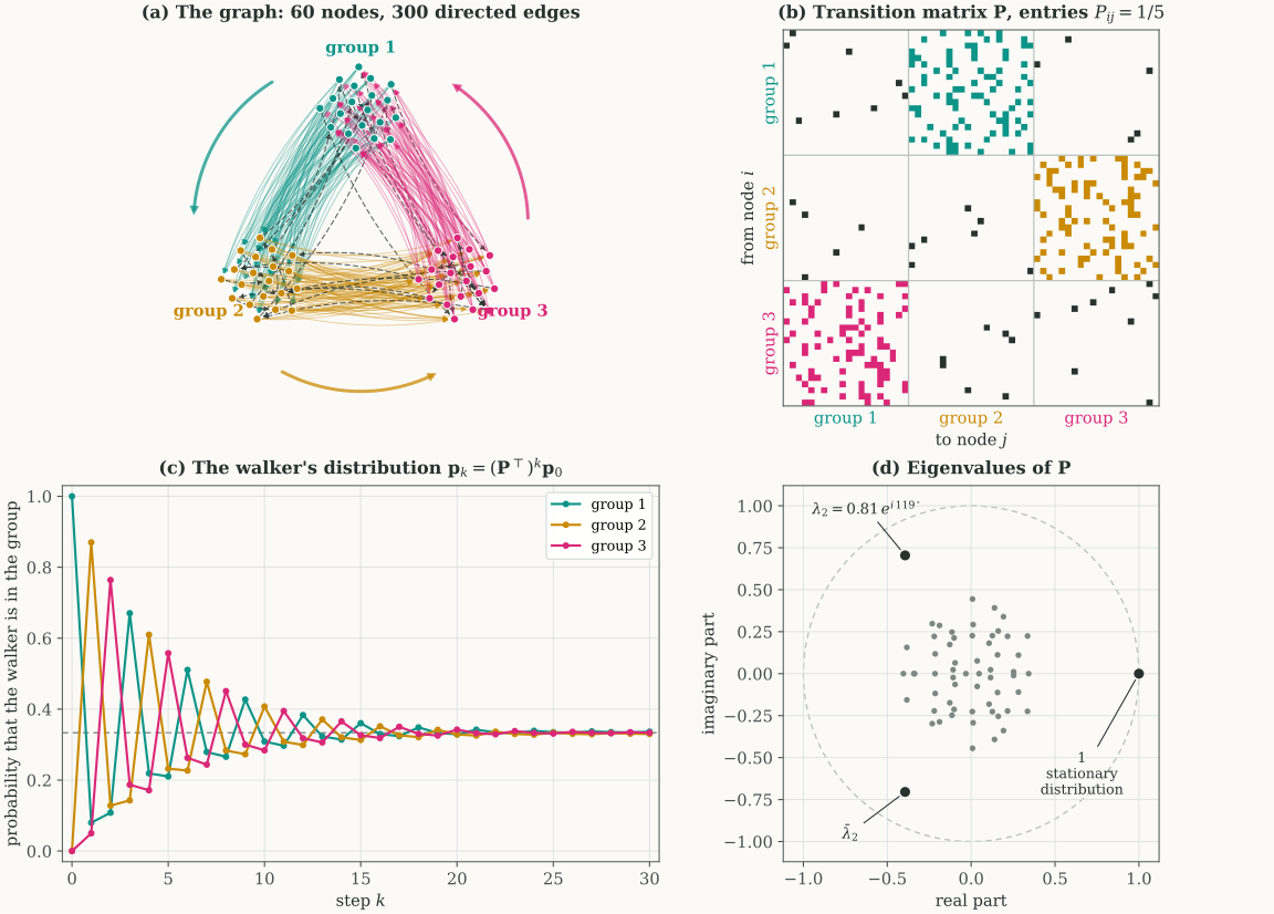
All these matrices are symmetric, and the results of Sections 3 and 4 rely on symmetry through the spectral theorem. For a nonsymmetric matrix accessed through products, such as the transition matrix of a random walk on a directed graph, whose entry (i,j) is the probability of stepping from node i to node j, the Arnoldi method (Arnoldi, 1951) replaces the Lanczos method. Section 5 presents it, together with nonsymmetric examples and what power iteration retains without symmetry.
3. Power iteration
In this part, we first establish the convergence conditions for ordinary power iteration, then describe how shifting and deflation recover additional eigenpairs. Starting from a unit vector v0, power iteration alternates a product with A and a normalization:
vk+1=∥Avk∥Avk,k≥0.
If Av0=0, then v0 is already an eigenvector with eigenvalue zero. In this case, the algorithm should return (0,v0) without attempting to normalize Av0.
The numerical analyst Alston S. Householder attributed the first treatment of the method to Müntz (1913) in his book The Theory of Matrices in Numerical Analysis (1964), as recalled in the historical survey of Golub and van der Vorst (2000). Deflation schemes built on it were analyzed early on, for example by Osborne (1958). The eigenvalue estimate of power iteration is the For a unit vector v, the Rayleigh quotient v⊤Av is the curvature of x↦21x⊤Ax along v. It lies between λmin(A) and λmax(A). It equals λ for every unit vector v of the eigenspace Eλ, since Av=λv gives v⊤Av=λ∥v∥2=λ. The converse fails: v⊤Av=λ does not make v an eigenvector, except when λ is λmin(A) or λmax(A).vk⊤Avk.
3.1 Proposition 1 [Convergence of power iteration]
Let v0∈Rd be a unit vector, and define
Λ0={λ∈Λ(A):Πλv0=0}.
Thus, Λ0 contains precisely the eigenvalues whose eigenspaces have a nonzero component in the initialization. Suppose that Λ0 contains a nonzero eigenvalue λ⋆ satisfying ∣λ⋆∣>∣λ∣ for every λ∈Λ0∖{λ⋆}. The eigenvalue λ⋆ may have arbitrary multiplicity. Then the iteration
vk+1:=∥Avk∥Avk=∥Ak+1v0∥Ak+1v0,k≥0,
is well defined, and
(sgn(λ⋆))kvk⟶q⋆:=∥Πλ⋆v0∥Πλ⋆v0.
In particular,
Aq⋆=λ⋆q⋆,vk⊤Avk⟶λ⋆.
Remark 1 [Why the dominant component wins]
Recall that for every vector v∈Rd and every integer k≥0,
v=∑λ∈Λ(A)Πλv and
Akv=∑λ∈Λ(A)λkΠλv.
So, for the iteration above, each application of A multiplies the component of the current vector in Eλ by λ, so after k steps the component in Eλ carries the factor λk:
Among the components present in v0, the blue one, with the largest ∣λ∣ (we have ∣λ⋆∣>∣λ∣ for every λ∈Λ0∖{λ⋆} by assumption), grows fastest, and the normalization removes the common factor ∣λ⋆∣k, so the orange components fade relative to it. Only the sign of λ⋆k survives, which is why the statement multiplies vk by (sgn(λ⋆))k. The limit is the normalized projection of v0 onto the whole eigenspace Eλ⋆: inside a repeated eigenspace, the direction is chosen by the initialization, not by the method.
Proof
Set pλ=Πλv0. The spectral decomposition gives
v0=λ∈Λ0∑pλ,Akv0=λ∈Λ0∑λkpλ(k≥1).
Well-definedness. Because pλ⋆=0 and λ⋆=0, the component
Πλ⋆Akv0=λ⋆kpλ⋆
is nonzero for every k≥0. Consequently, Akv0=0 for every k≥0. Since ∥v0∥=1, repeated normalization satisfies
vk=∥Akv0∥Akv0.
Indeed, this identity holds at k=0. If it holds at iteration k, then
The blue term is the component along the dominant eigenspace, and it keeps its size after rescaling. The orange term collects every other component, and it shrinks geometrically. Since pλ⋆∈Eλ⋆, the limit q⋆ satisfies Aq⋆=λ⋆q⋆.
Rayleigh quotient. For k≥1, the symmetry of A and its spectral decomposition A=∑λ∈Λ(A)λΠλ give
The second line uses (Akv0)⊤=v0⊤Ak, since A is symmetric. The third expands A2k+1 and A2k with Aj=∑λλjΠλ. The fourth uses v0⊤Πλv0=v0⊤Πλ⊤Πλv0=∥Πλv0∥2=∥pλ∥2, which holds because Πλ is symmetric and Πλ2=Πλ, and only the eigenvalues of Λ0 remain, since pλ=0 for the others. The fifth divides the numerator and the denominator by λ⋆2k>0.
■□
Remark 2 [A negative dominant eigenvalue]
If λ⋆>0, Proposition 1 gives vk→q⋆. If λ⋆<0, it gives (−1)kvk→q⋆, or, equivalently,
v2k⟶q⋆ and v2k+1⟶−q⋆.
Thus, in the latter case, the even and odd subsequences converge to opposite unit vectors. The raw sequence {vk}k≥0 does not converge, but min{∥vk−q⋆∥,∥vk+q⋆∥}⟶0.
A stopping rule that compares consecutive iterates, such as ∥vk+1−vk∥≤ε with ε<2, is therefore eventually never satisfied when λ⋆<0, because ∥vk+1−vk∥→2∥q⋆∥=2, even though the eigendirection has converged. The Rayleigh quotient converges in both cases.
3.2 Theorem 1 [Rate of convergence]
Assume the hypotheses of Proposition 1, and write pλ⋆=Πλ⋆v0. Let ρ2=max{∣λ∣:λ∈Λ0∖{λ⋆}},
with ρ2=0 when Λ0={λ⋆}, and let ϕ0∈[0,π/2) be Write v0=pλ⋆+(v0−pλ⋆), where pλ⋆=Πλ⋆v0 lies in Eλ⋆ and the remainder is orthogonal to it. The three vectors form a right triangle: the hypotenuse v0 (black), a side pλ⋆ along Eλ⋆ (blue), and a side v0−pλ⋆ perpendicular to it (orange). The angle between a vector and a subspace is the angle between the vector and its orthogonal projection, the smallest angle it makes with a vector of the subspace, so ϕ0 is the angle between v0 and pλ⋆. The tangent is the opposite side over the adjacent side, and since ∥v0∥=1, also cos(ϕ0)=∥pλ⋆∥ and sin(ϕ0)=∥v0−pλ⋆∥. The hypothesis pλ⋆=0 keeps ϕ0 below π/2., so that tan(ϕ0)=∥v0−pλ⋆∥/∥pλ⋆∥. Then, for every k≥1,
Relative to the dominant component, each product multiplies the component in Eλ by λ/λ⋆ (Remark 1), so the slowest of them, with ∣λ∣=ρ2, sets the pace. The eigenvector error therefore shrinks by the factorρ2/∣λ⋆∣ per product, and the eigenvalue error by its square, because the Rayleigh quotient is stationary at an eigenvector. The factor can be arbitrarily close to one. Remark 5 below is the limiting case ρ2=∣λ⋆∣, in which convergence can fail altogether.
Proof
Recall from the proof of Proposition 1 the scaled remainder and the normalized iterate:
The vectors pλ lie in mutually orthogonal eigenspaces, so the squared norm of a combination of them is the sum of the squared norms of its terms (Pythagoras). Every ∣λ∣ in the sum defining rk is at most ρ2, hence
where the last equality is Pythagoras again, applied to v0−pλ⋆=∑λ=λ⋆pλ.
Write tk=∥rk∥/∥pλ⋆∥, so that tk≤(ρ2/∣λ⋆∣)ktan(ϕ0).
Since rk is orthogonal to pλ⋆ and q⋆=pλ⋆/∥pλ⋆∥, the inner product of the unit vector (sgn(λ⋆))kvk with q⋆ is
For unit vectors w and q, ∥w−q∥2=∥w∥2−2w⊤q+∥q∥2=2−2w⊤q, so
(sgn(λ⋆))kvk−q⋆2=2−1+tk22≤tk2,
because 1/1+t≥1−t/2 for all t≥0 (the convex function t↦1/1+t lies above its tangent line at 0). Taking square roots and using the bound on tk gives the first inequality. For the Rayleigh quotient, recall the fifth line of the Rayleigh-quotient display in the proof, whose denominator equals ∥pλ⋆∥2+∥rk∥2 by the expression of ∥rk∥2 above:
The first inequality moves the absolute value inside the sum (triangle inequality). The second uses ∣λ−λ⋆∣≤∣λ∣+∣λ⋆∣<2∣λ⋆∣, since every other eigenvalue present satisfies ∣λ∣<∣λ⋆∣, and makes the denominator smaller by dropping ∥rk∥2. The two equalities are the expression of ∥rk∥2 above and the definition of tk, and the last inequality squares the bound on tk. This is the second inequality of the theorem.
■□
Remark 4 [Which eigenvalue is found]
The hypothesis of Proposition 1 concerns distinct eigenvalues present in the initialization. It does not require the dominant eigenvalue to be simple, since the limit is the normalized projection of v0 onto its entire eigenspace. To obtain an eigenvalue of globally largest absolute value, the initialization must have a nonzero projection onto a corresponding eigenspace. For example, if
v0=g/∥g∥ with
g∼N(0,Id),
then Πλv0=0 for every λ∈Λ(A) with probability one. Indeed, for each λ, the event Πλg=0 means that g belongs to the proper linear subspace Eλ⊥, which has A proper subspace S lies in a hyperplane {x:c⊤x=0} with c=0. For g∼N(0,Id), the number c⊤g is Gaussian with variance ∥c∥2>0, so it equals zero with probability zero.. There are only finitely many eigenspaces. Consequently, such an initialization satisfies the hypotheses of Proposition 1 whenever A=0 and exactly one distinct eigenvalue of A has maximal absolute value.
Remark 5 [Failure for opposite eigenvalues of equal dominant magnitude]
The condition examined here is the strict dominance assumption of Proposition 1. In words, some nonzero eigenvalue present in the initialization is strictly larger in absolute value than every other eigenvalue present. With Λ0={λ∈Λ(A):Πλv0=0}, the set of eigenvalues present, it reads
∃λ⋆∈Λ0∖{0}∀λ∈Λ0∖{λ⋆}:∣λ⋆∣>∣λ∣.
The condition fails when no eigenvalue present stands out in this way: every nonzero eigenvalue present is matched or exceeded in absolute value by another eigenvalue present. Negating the statement above gives
∀μ∈Λ0∖{0}∃λ∈Λ0∖{μ}:∣λ∣≥∣μ∣.
Suppose that the condition fails, while some nonzero eigenvalue is present in the initialization. Let ρ=max{∣λ∣:λ∈Λ0} be the largest absolute value among the eigenvalues present, so that ρ>0. If only one element of Λ0 had absolute value ρ, it would be strictly larger in absolute value than every other eigenvalue present, and the condition would hold with λ⋆ equal to that element. Since the condition fails, at least two distinct elements of Λ0 have absolute value ρ, +ρ and −ρ, and both are present in the initialization. We show that ordinary power iteration can then fail to converge to any eigendirection, even while its Rayleigh quotient converges.
Suppose that
p+=Πρv0=0,p−=Π−ρv0=0;
and that every other eigenvalue present in v0 has absolute value smaller than ρ. For k≥1, define the scaled remainder
rk=λ∈Λ0∣λ∣<ρ∑(ρλ)kpλ.
Then
∥rk∥2=λ∈Λ0∣λ∣<ρ∑ρλ2k∥pλ∥2⟶0,
and
vk=∥p+∥2+∥p−∥2+∥rk∥2p++(−1)kp−+rk.
The blue component keeps its sign, the orange component changes sign at every step, and the remainder vanishes. Hence
v2k⟶∥p+∥2+∥p−∥2p++p−,
whereas
v2k+1⟶∥p+∥2+∥p−∥2p+−p−.
These two limits are not collinear. Indeed, if p++p−=c(p+−p−) for some scalar c, projecting onto Eρ gives c=1, whereas projecting onto E−ρ gives c=−1. Thus no choice of an overall factor in {−1,1} can make the iterates converge to a single unit eigenvector.
Nevertheless, the Rayleigh quotient satisfies
This limit need not be an eigenvalue. For example, let
A=[100−1],v0=21[11].
Then, at every iteration,
vk=21[1(−1)k],vk⊤Avk=0.
However,
0∈/Λ(A),Avk−(vk⊤Avk)vk=∥Avk∥=1.
Thus a constant or convergent Rayleigh quotient does not by itself establish convergence to an eigenpair. This obstruction motivates the squared-power construction of Proposition 2 below and the use of an eigenpair residual as a stopping criterion.
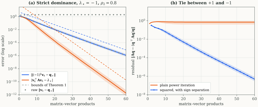
Figure 1. Power iteration on two symmetric matrices of size d=60 with random eigenvectors. Each curve is the median over 200 Gaussian initializations, and its band contains the middle half of the runs (the interquartile range). (a) The dominant eigenvalue λ⋆=−1 has multiplicity 3 and the next largest magnitude is ρ2=0.8. The sign-corrected error ∥(−1)kvk−q⋆∥ (blue) decays like 0.8k and the Rayleigh-quotient error (orange) like 0.82k, below the bounds of Theorem 1 (dashed), while the raw distance ∥vk−q⋆∥ (grey) alternates between those small values and nearly 2 (Remark 2). (b) The eigenvalues +1 and −1 tie for the largest magnitude. The residual ∥Av−(v⊤Av)v∥ of plain power iteration (orange) stalls at order one (Remark 5), whereas squared power iteration with sign separation (blue; Proposition 2, run as in Algorithm 1) drives the residual of its candidate to zero, by a factor of about 0.8 per product. Both horizontal axes count matrix–vector products: vk costs k products and its Rayleigh quotient one more, and each squared step costs two.
3.3 Corollary 1 [Recovering algebraic extrema by shifting]
Let λmin=minΛ(A) and λmax=maxΛ(A).
If α≥λmax and α>λmin, then power iteration applied to B=αId−A converges to a unit vector in Eλmin, provided its initialization has a nonzero projection onto that eigenspace. Its Rayleigh quotient converges to μmax=α−λmin, so λmin=α−μmax.
Similarly, if β≤λmin and β<λmax, then power iteration applied to C=A−βId converges to a unit vector in Eλmax, provided its initialization has a nonzero projection onto that eigenspace. Its Rayleigh quotient converges to νmax=λmax−β, so λmax=β+νmax.
Remark 6 [What a shift does to the spectrum]
Power iteration returns the eigenvalue of largest magnitude, which is λmax or λmin depending on the signs. A scalar shift moves the whole spectrum without changing the eigenvectors, and the shift αId−A also reverses its order. With α≥λmax, the spectrum of B lies in [0,α−λmin], so the eigenvalue of A farthest below α becomes the dominant eigenvalue of B.
Proof
For any eigenpair (λ,u) of A,
Bu=(αId−A)u=(α−λ)u.
Since an orthonormal eigenbasis of A is also an eigenbasis of B,
Λ(B)={α−λ:λ∈Λ(A)}.
The assumptions on α give
0≤α−λ≤α−λmin and
α−λmin>0.
Whenever λ>λmin, α−λ<α−λmin.
Therefore, B has a positive dominant eigenvalue α−λmin, whose eigenspace is exactly Eλmin. Proposition 1 applies, including when this eigenvalue is repeated.
For C,
Cu=(A−βId)u=(λ−β)u
and Λ(C)={λ−β:λ∈Λ(A)}.
The assumptions on β give
0≤λ−β≤λmax−β
and λmax−β>0.
Whenever λ<λmax, λ−β<λmax−β.
Thus C has a positive dominant eigenvalue λmax−β, with eigenspace Eλmax. Proposition 1 again applies.
■□
In particular, choosing α=λmax recovers the minimum eigenvalue from the maximum, unless A=λmaxId. In that exceptional case, every eigenvalue already equals λmax. The analogous statement holds for β=λmin.
Remark 7 [The shift only needs to pass the midpoint]
The condition α≥λmax is convenient but stronger than needed. Proposition 1 only requires that α−λmin strictly dominate ∣α−λ∣ for every other eigenvalue λ present in the initialization. For λ≤α, this holds because λ>λmin. For λ>α, it reads λ−α<α−λmin, that is, λ+λmin<2α. Hence every shift α>(λmin+λmax)/2 works. In particular, an underestimate of λmax, such as a Rayleigh quotient, is a valid shift as long as it exceeds the midpoint of the spectrum. Symmetrically, every β<(λmin+λmax)/2 works for C.
A scalar shift changes every eigenvalue. It does not generally make the next eigenvalue in a prescribed ordering dominant. Deflation does. Power iteration finds one eigenpair, the dominant one, and running it again on A would only find the same pair. To reach the next pair, deflation removes from A the eigendirections already found and leaves every other eigenpair untouched. In an orthonormal eigenbasis q1,…,qd of A, with Aqi=λiqi, the spectral decomposition writes A as a sum of rank-one layers, one per eigenvector, and deflating the first r eigenvectors means deleting their layers, which gives a new matrix, the deflated matrix B:
This matrix has the same eigenvectors as A. The ones already found (orange) now have the eigenvalue 0, and all the others (blue) keep their eigenvalues. The largest remaining eigenvalue of A in absolute value is therefore the dominant eigenvalue of B, and power iteration on B finds it. The layer picture uses every eigenvector, but computing B does not: the lemma below shows that it only needs the eigenvectors already found, through the projection P=Id−QQ⊤ that removes the components along them.
3.4 Lemma 1 [Orthogonal deflation]
Let q1,…,qr be exact orthonormal eigenvectors of A, with associated eigenvalues λ1,…,λr:
Aqi=λiqi,qi⊤qℓ=δiℓ,i,ℓ∈{1,…,r}.
Define
Q=[q1,…,qr],D=diag(λ1,…,λr),P=Id−QQ⊤.
Then
B=PAP=A−QDQ⊤=A−i=1∑rλiqiqi⊤.
Moreover,
The eigenvectors already found have the eigenvalue 0 for B. For each column qi of Q, Bqi=0, for i∈{1,…,r}.
On the vectors orthogonal to the eigenvectors already found, B acts exactly as A. That is, Bx=Ax for every x with Q⊤x=0, which is to say for every x∈range(P)=span{q1,…,qr}⊥.
The other eigenpairs of A are eigenpairs of B. Every eigenvector of A orthogonal to q1,…,qr is an eigenvector of B with the same eigenvalue. Hence the restriction of B to range(P)=span{q1,…,qr}⊥ has the remaining eigenvalues of A, counted with multiplicity, and B has the eigenvalue 0 on span{q1,…,qr}.
Remark 8 [Two views of the deflated matrix]
The two formulas for B are two ways of computing a product Bx with one product by A.
Projection,Bx=P(A(Px)): remove from x its components along the stored eigenvectors, apply A, and remove those components again. A vector orthogonal to every stored eigenvector passes through unchanged (item 2), and a stored eigenvector is sent to 0 (item 1).
Subtraction,Bx=Ax−∑i=1rλi(qi⊤x)qi: apply A, then subtract the layers of the stored eigenpairs, exactly as in the picture above.
The two agree because the qi are exact eigenvectors, and the proof below uses AQ=QD. For computed, approximate eigenvectors they differ. The projection still returns vectors exactly orthogonal to the stored ones, so the eigenvectors found later stay orthogonal to them, which is why the implementation below applies P explicitly.
Extend q1,…,qr to an orthonormal eigenbasis q1,…,qd of A. For every i>r,
Q⊤qi=0,Bqi=Aqi=λiqi.
Thus the eigenpairs associated with qr+1,…,qd are preserved on range(P).
■□
When an eigenvalue is repeated, deflating one unit eigenvector removes only that direction. Other directions in the same eigenspace that are orthogonal to it retain their eigenvalue.
Ordinary power iteration can be applied repeatedly to the deflated operator whenever the hypotheses of Proposition 1 hold at each stage. The following modification also handles opposite eigenvalues of equal magnitude, without requiring a spectral bound.
3.5 Proposition 2 [Power iteration with sign separation]
Let B∈Rd×d be symmetric, and let w0 be any unit vector. If Bw0=0, then (0,w0) is an eigenpair. Otherwise, the iteration
wk+1=∥B2wk∥B2wk
is well defined and converges to a unit vector w satisfying
B2w=ρ2w
for some ρ>0. This value can be recovered as
ρ=∥Bw∥.
Define
u+=21(w+ρBw),u−=21(w−ρBw).
Then
Bu+=ρu+,Bu−=−ρu−.
At least one of u+ and u− is nonzero. Normalizing either nonzero vector gives an eigenvector of B.
Remark 9 [Sign separation is a reflection]
Squaring maps +ρ and −ρ to the same eigenvalue ρ2 of B2, so the obstruction of Remark 5 disappears: B2 is positive semidefinite, and its largest eigenvalue present in w0 is strictly dominant. The price is that the limit w may mix the two eigenspaces of B for +ρ and −ρ. One more product separates them. The limit lies in the eigenspace of B2 for ρ2, which is the sum of these two eigenspaces, so we can write w=w++w− with Bw±=±ρw±. Then Bw/ρ=w+−w− is the On the sum of the two eigenspaces, B/ρ fixes every vector of the +ρ eigenspace and reverses every vector of the −ρ eigenspace: it is the mirror reflection across the +ρ eigenspace. Averaging a vector with its mirror image keeps its part on the mirror; averaging it with minus its mirror image keeps the other part. of w that fixes the blue part and reverses the orange part, so
u+=w+,u−=w−
are exactly the orthogonal projections of w onto the two eigenspaces. The orthogonality and norm identities in the proof below are this observation written out.
Proof
Let ΠλB denote the orthogonal projection onto the eigenspace of B associated with λ. Since Bw0=0, the initialization has a nonzero component in at least one nonzero eigenspace of B. Define
ρ=max{∣λ∣:λ∈Λ(B),ΠλBw0=0}>0.
The eigenvalues of B2 are the numbers λ2. Its largest eigenvalue present in w0 is therefore ρ2>0, and every other distinct eigenvalue present is strictly smaller than ρ2.
Proposition 1, applied to B2, shows that the iterates are well defined and converge to a unit vector w in the eigenspace associated with ρ2:
B2w=ρ2w.
Also,
u++u−=w=0,
so the two vectors cannot both be zero. More precisely,
u+⊤u−=41(∥w∥2−ρ2∥Bw∥2)=0,
and
∥u+∥2+∥u−∥2=1.
Therefore,
max{∥u+∥,∥u−∥}≥1/2.
Choosing the vector with larger norm avoids normalizing a potentially very small component.
■□
This construction does not require forming B2. Its action is obtained through B2x=B(Bx), using two applications of B. Squaring removes the distinction between the eigenvalues +ρ and −ρ during power iteration. The subsequent construction of u+ and u− separates their eigenspaces.
3.6 Corollary 2 [Recovery of a complete eigenbasis]
For every real symmetric matrix A, orthogonal deflation combined with Proposition 2 recovers a complete orthonormal eigenbasis, including repeated and zero eigenvalues, when each inner power iteration is taken to its limit. The procedure is as follows.
Initialize Q0∈Rd×0 as an empty matrix, that is, a matrix with no columns, so that Q0Q0⊤=0d×d (each entry is an empty sum).
At stage j∈{1,…,d}, define Pj−1=Id−Qj−1Qj−1⊤ and Bj=Pj−1APj−1. Choose z such that Pj−1z=0, and set w0=Pj−1z/∥Pj−1z∥. For example, a fresh draw z∼N(0,Id) gives a nonzero denominator with probability one.
If Bjw0=0, set qj=w0 and λj=0. Otherwise, apply Proposition 2 to Bj, choose the larger of the two sign-separated components in norm, and normalize it to obtain qj. Recover the eigenvalue as λj=qj⊤Aqj.
Append the new eigenvector, Qj=[Qj−1,qj], and continue to the next stage.
Proof
At the first stage, P0=Id and B1=A, so Proposition 2 yields an eigenpair of A.
Suppose that the first j−1 stages have produced orthonormal eigenvectors of A. By Lemma 1,
Bjx=Ax whenever Qj−1⊤x=0.
The initialization belongs to this orthogonal complement. Since Bj=Pj−1APj−1, every squared-power iterate also belongs to it. The limit vector and the sign-separated vectors therefore belong to it as well.
Consequently, the resulting unit vector qj satisfies
Aqj=Bjqj=λjqj and
Qj−1⊤qj=0.
The zero case is also valid: if Bjw0=0, then
Aw0=Bjw0=0.
Thus each stage adds one unit eigenvector orthogonal to all previously stored eigenvectors.
After d stages,
Qd⊤Qd=Id and
AQd=Qddiag(λ1,…,λd).
Since the square matrix Qd is orthogonal, QdQd⊤=Id, and hence
A=Qddiag(λ1,…,λd)Qd⊤.
■□
Any admissible nonzero initialization suffices to recover some eigenpair at each stage. With fresh Gaussian initializations, the procedure selects an eigenvalue of largest remaining absolute value with probability one. Consequently, the eigenvalues are obtained in nonincreasing absolute value, with arbitrary ordering within ties. Algebraic ordering can be obtained by sorting afterward.
The exact test Bjw0=0 identifies a zero eigenvector. It does not require concluding that the entire remaining operator is zero.
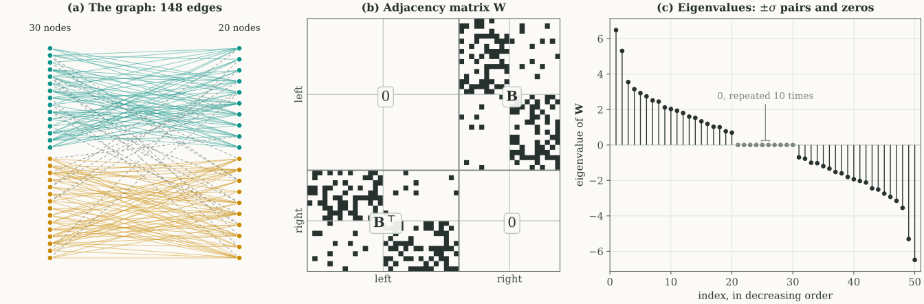
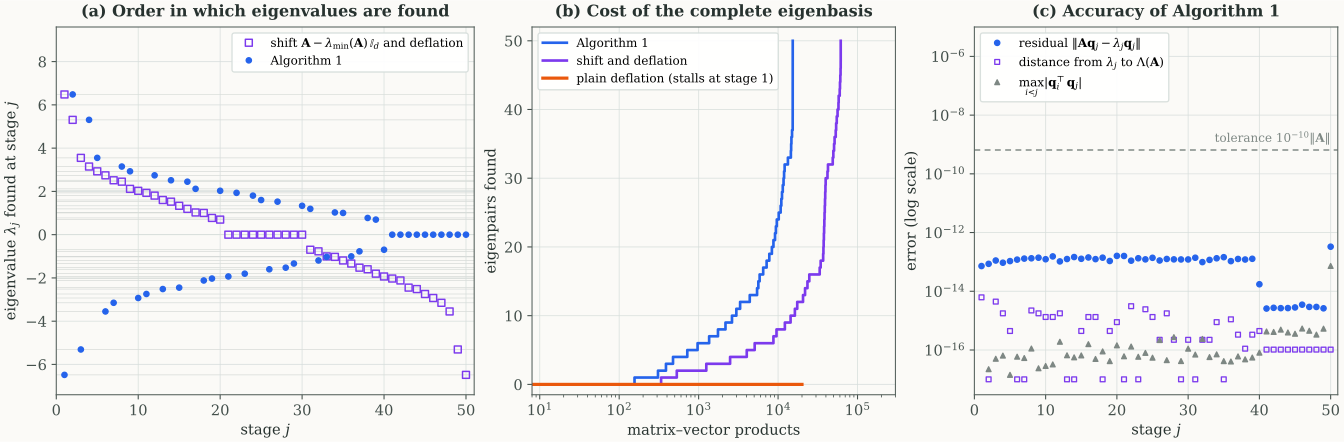
Figure 2 below shows the adjacency matrix of a bipartite graph, whose nonzero eigenvalues come in opposite pairs and whose eigenvalue 0 is repeated. Figure 3 runs this procedure on it and compares it with deflation combined with ordinary power iteration, with and without a shift.
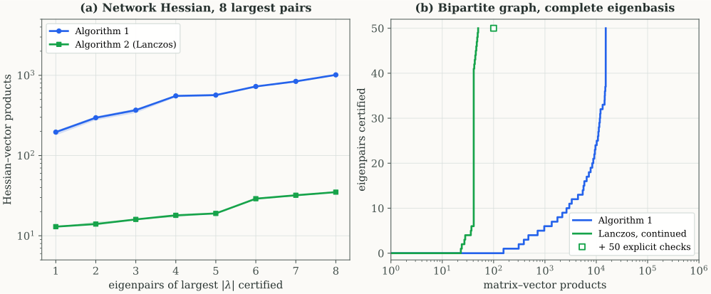
Figure 2. The bipartite graph used in Figures 3 and 7. (a) The graph has 30 nodes on one side and 20 on the other, each side split into two planted communities (teal and gold). Each of the 30×20 possible edges between the two sides is present with probability 0.45 when the communities match and 0.08 otherwise, and no edge joins two nodes of the same side. The draw has 148 edges, 128 within communities (colored) and 20 across (grey, dashed). (b) Its adjacency matrix W, with the nodes ordered side by side and community by community. The diagonal blocks are zero, and the off-diagonal blocks are the 30×20 biadjacency matrix B and its transpose, so a product Wx is one pass over the 148 edges. (c) The 50 eigenvalues of W in decreasing order. They are symmetric about 0. Writing a vector of R50 as (x,y) with x∈R30 and y∈R20, W(x,y)=(By,B⊤x), so a pair of singular vectors with Bv=σu and B⊤u=σv gives the eigenvector (u,v) for σ and (u,−v) for −σ. The 20 singular values of B give the 40 nonzero eigenvalues, and 0 is repeated 30−20=10 times.Figure 3. A complete eigenbasis of the adjacency matrix of the bipartite graph of Figure 2, applied through its edge list (Section 2.2). Because the graph is bipartite, every nonzero eigenvalue σ comes with −σ, so plain power iteration meets the tie of Remark 5 at once, and 0 is an eigenvalue of multiplicity 10. Every stage starts from a fresh Gaussian vector and, as in Corollary 2, is taken to its limit: it runs until the residual of its candidate for the deflated matrix Bj is below 10−13. (a) Eigenvalue found at each stage. Algorithm 1 (blue) finds the eigenvalues in nonincreasing absolute value, the two members of each pair at consecutive stages, and the ten zero eigenvalues last. Power iteration on A−λmin(A)Id with deflation (purple; Corollary 1 and Lemma 1) finds them in decreasing order. Grey lines mark the 41 distinct eigenvalues. (b) Number of eigenpairs found against the number of products. Algorithm 1 uses 15,296 products in all, two for each zero eigenvalue. The shifted iteration uses 61,453, even with the most favorable shift λmin(A)=−6.48: adding 6.48 to every eigenvalue brings the ratios that set the speed of convergence (Theorem 1) closer to one, and each zero eigenvalue takes a full stage. Plain deflated power iteration (orange) never completes its first stage, and after 20,000 products its residual is still above 1.9. (c) Accuracy of the eigenbasis of Algorithm 1, far below the tolerance 10−10∥A∥ (grey, dashed): residuals (blue) below 3.3⋅10−13, eigenvalues within 6.3⋅10−15 of the spectrum (purple; exact zeros drawn at 10−17), inner products between distinct eigenvectors (grey) below 7.3⋅10−14, and ∥A−Q50diag(λ1,…,λ50)Q50⊤∥=2.2⋅10−13.
3.7 Lemma 2 [Residual certificate for an approximate eigenpair]
For any unit vector q, define
λ=q⊤Aq
and
r=Aq−λq.
Then minλ∈Λ(A)∣λ−λ∣≤∥r∥.
Remark 10 [A computable bound on an unknown distance]
The residual is computable with one product, and it bounds an unknown quantity: the distance from the estimate λ to the nearest true eigenvalue. If q is exactly an eigenvector, the residual is zero, and the bound says that λ is exactly an eigenvalue.
Proof
Expand q in an orthonormal eigenbasis u1,…,ud of A:
The squared residual is thus an average of the squared distances from λ to the eigenvalues, with weightsci2 that sum to one, so it is at least the smallest of them. Taking square roots gives the result.
■□
This certificate concerns proximity to some eigenvalue. A small residual alone does not certify that the eigenvalue has the largest remaining absolute value.
Remark 11 [Any scalar, and the best one]
The proof never uses the definition of λ. The same expansion gives
λ∈Λ(A)min∣μ−λ∣≤∥Aq−μq∥for every scalar μ,
so the certificate applies to an eigenvalue estimate computed by any means, as long as it is paired with a unit vector. The Rayleigh quotient is the best choice of μ. Indeed, expanding the square with ∥q∥=1 and λ=q⊤Aq gives
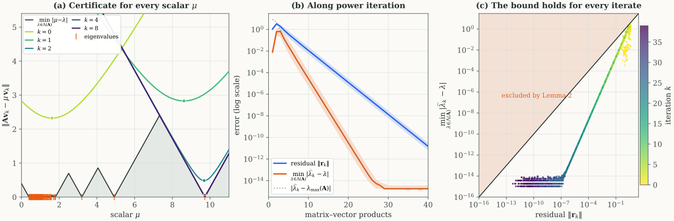
where the last line is the second one at μ=λ. The blue term does not depend on μ, so the certificate is smallest at μ=λ, where it equals the residual of Lemma 2, and the orange term is the price of any other estimate. As a function of μ, the certificate (μ−λ)2+∥r∥2 is a hyperbola centered at the Rayleigh quotient, and it lies above the distance from μ to the spectrum, as panel (a) of Figure 4 below shows.
Figure 4. The residual certificate on the sample covariance matrix n1X⊤X of n=400 centered observations of d=60 variables, applied as X⊤(Xv)/n (Section 2.2). Its three largest eigenvalues, the variances along the first three principal components, are 9.72, 4.92 and 3.20, and the other 57 lie in [0.40,1.80]. (a) For the iterates vk of power iteration from one Gaussian start, the certificate μ↦∥Avk−μvk∥ of Remark 11 (light to dark as k grows) lies above the distance from μ to the spectrum (black, with the eigenvalues marked in orange on the axis) for every scalar μ. Its minimum, marked by a dot, is attained at the Rayleigh quotient λk and equals the residual ∥rk∥ of Lemma 2. (b) Medians over 200 Gaussian starts, with bands containing the middle half of the runs. The residual (blue) shrinks by the factor λ2/λ1≈0.51 per product, and the distance from λk to the nearest eigenvalue (orange) by its square (Theorem 1), until rounding errors of order 10−15 stop it. The certificate is valid but pessimistic: after 20 products, the median residual is 1.2⋅10−5 and the median distance 3.2⋅10−11. In the first steps, λk lies among the small eigenvalues, and its distance to the nearest of them (orange) is much smaller than its distance to λmax(A) (grey, dotted): the certificate concerns some eigenvalue, not necessarily the largest. (c) The pairs formed by the residual and the distance for 50 runs, colored by k from light to dark. None lies above the diagonal, as Lemma 2 requires, and over all 200 runs and 40 steps the largest ratio of the distance to the residual is 0.995. Distances below 10−15, at rounding level, are drawn at 10−15.
3.8 Algorithm 1 [Deflated squared power iteration with sign separation]
For a finite implementation, squared power iteration and sign separation can be combined without explicitly constructing A, P or B. At a given deflation stage, let Q contain the previously computed orthonormal vectors, and implement the projection through
Px=x−Q(Q⊤x).
Choose tolerances εabs>0 and εrel≥0. Starting from a unit vector w satisfying Q⊤w=0, repeat the following steps.
First product. Compute h1=Aw, a=Ph1 and ρ=∥a∥. If ρ=0, go to step 5.
Second product. Set y=a/ρ, then compute h2=Ay and b=Ph2.
Candidate. Choose the scalar sign s=+1 if w⊤y≥0 and s=−1 if w⊤y<0. This selects whichever of w+y and w−y has larger norm. Form n=∥w+sy∥ and q=(w+sy)/n. The product of the candidate with the original matrix is available by linearity: Aq=(h1+sh2)/n.
Check or update. Compute λ=q⊤Aq and r=Aq−λq. If ∥r∥≤εabs+εrel∥Aq∥, accept (λ,q) and append q to Q. Otherwise, update w←b/∥b∥ and return to step 1.
Zero projected product. If ρ=0, use q=w as the candidate, compute λ=q⊤Aq and r=Aq−λq, where Aq=h1, and check the same original residual before accepting the pair.
■□
Because w and y are unit vectors, the normalization in step 3 is never small:
n2=∥w∥2+∥y∥2+2sw⊤y=2+2∣w⊤y∣≥2.
For the symmetric projected operator B=PAP, these operations satisfy
a=Bw,y=ρBw,b=ρB2w,
because Pw=w and Py=y. Thus the update is normalized power iteration on B2, with a normalized intermediate vector. In exact arithmetic, ρ>0 implies b=0, because
w⊤B2w=∥Bw∥2=ρ2>0.
The sign separation is meaningful before exact convergence. For a unit vector w with
ρ=∥Bw∥>0,n=w+sρBw,q=nw+sBw/ρ,
direct calculation gives
(B−sρId)q=nBw+sB2w/ρ−sρw−Bw=ρns(B2w−ρ2w).
The blue terms cancel because s2=1. Since n≥2, the eigenpair residual of the candidate for B is at most ∥B2w−ρ2w∥/(2ρ). Thus, as squared power iteration converges, the extracted candidate becomes an eigenvector of B. The stopping criterion nevertheless uses the original residual Aq−λq, because numerically computed deflation vectors need not span an exactly invariant subspace of A.
In step 5, a small computed value of ρ does not establish that every remaining eigenvalue is zero. This is why the zero case is also accepted only through the original residual.
In floating-point arithmetic, the implementation should reorthogonalize projected vectors, impose a maximum number of inner iterations, and report nonconvergence if the original residual does not reach the requested tolerance. No vector with computed norm zero should be normalized. A numerical breakdown should instead trigger a residual check, a restart, or a report of nonconvergence.
The exact recovery guarantee of Corollary 2 concerns limiting iterates and exact deflation. With approximate deflation vectors, convergence for PAP need not drive the residual for the original matrix A below an arbitrarily small tolerance. Finite computations therefore return approximate eigenpairs whose original residuals must be checked.
The residual for A splits exactly into a part that the inner iteration reduces and a part that it inherits. Let λ1,…,λr be the eigenvalue estimates of the stored pairs, and let the columns of R=AQ−Qdiag(λ1,…,λr) be their residuals. For a unit candidate q with Q⊤q=0 and λ=q⊤Aq, we have Pq=q, hence Aq=Bq+QQ⊤Aq, where Bq−λq lies in range(P) and QQ⊤Aq in range(Q). Since Q⊤q=0, we also have Q⊤Aq=(AQ)⊤q=R⊤q. The two parts are orthogonal, so
∥Aq−λq∥2=∥Bq−λq∥2+∥R⊤q∥2.
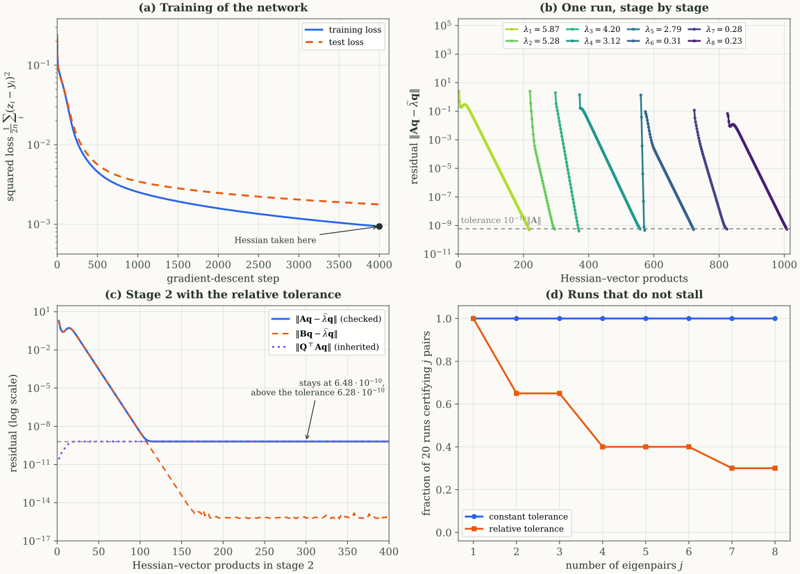
The inner iteration drives the orange term to zero. The purple term is inherited from the stored pairs: each entry of R⊤q is the inner product of q with a stored residual, so the term is at most the sum of their squared norms, but nothing in the inner iteration makes it small. A stage therefore stalls when its threshold εabs+εrel∥Aq∥ is below the inherited part. This happens readily with εrel>0, because the threshold shrinks with ∣λ∣, whereas the inherited part comes from earlier stages, whose eigenvalues are larger in absolute value and whose accepted residuals can be nearly as large as their own thresholds. A threshold that is the same at every stage (εrel=0) removes this systematic mismatch, but over many stages the inherited parts can still exceed it. Continuing each stage until the residual for B reaches rounding level, and only then checking the residual for A, keeps every inherited part far below the threshold, at the price of more products. Figure 5 below shows the stall on the Hessian of a neural network. The complete eigenbasis in Figure 3 was computed in the last way. With the same constant threshold but without the continuation, that run stalls at stage 20 of 50, where the inherited part is 6.89⋅10−10 and the threshold 6.48⋅10−10.
Figure 5.Algorithm 1 on the Hessian of a training loss, applied by automatic differentiation (Section 2.1). The network is a fully connected tanh network with layer widths 4, 16, 16 and 1, so that θ∈R369, trained by 4,000 steps of gradient descent on n=256 Gaussian inputs labelled by a random teacher network, down to a squared loss of 9.4⋅10−4. Its Hessian has five large eigenvalues, from 5.87 down to 2.79, the next ones are near 0.3, and 147 of its eigenvalues are negative but above −0.0023. Algorithm 1 computes the 8 eigenpairs of largest absolute value with two threshold rules: a constant one, εabs=10−10∥A∥ and εrel=0, where ∥A∥=5.87 is the absolute value of the first eigenvalue found, and a relative one, εabs=εrel=10−10. (a) The squared losses along the 4,000 steps of gradient descent, on the training inputs (blue) and on 1,024 fresh inputs labelled by the same teacher (orange, dashed). The Hessian is taken at the last step (black dot), where the training loss is 9.4⋅10−4 and the test loss reaches its lowest value, 1.8⋅10−3. (b) One run with the constant threshold: the residual of the candidate against the cumulative number of Hessian–vector products, with the stages colored from light to dark and labelled by their eigenvalues. Each stage decreases geometrically, by a factor per product equal to the ratio of the next largest remaining absolute value to its own, until it reaches the threshold (grey, dashed), and the eight stages take 1,008 products. (c) A run with the relative threshold, at its second stage. The residual for A (blue), which the algorithm checks, splits into the residual for B (orange, dashed), which the inner iteration drives down to 5⋅10−16, and the inherited part ∥Q⊤Aq∥ (purple, dotted), which equals the residual 6.48⋅10−10 accepted at the first stage. The threshold of the second stage, 10−10(1+5.28)=6.28⋅10−10, is just below it, so the stage never stops. (d) Fraction of 20 runs, each with its own Gaussian starting vectors, that certify the j largest pairs. With the relative threshold (orange), 14 runs stall: 7 at stage 2, 5 at stage 4 and 2 at stage 7. With the constant threshold (blue), all 20 runs certify the 8 pairs, and in the run of panel (b) every eigenvalue is within 6⋅10−15 of the spectrum.
The operator must stay fixed for the whole run. For a Hessian A=∇θ2f(θ), each product is computed as in Section 2.1, with θ and everything that defines f held fixed.
Each nondegenerate inner iteration above uses two matrix–vector products, h1 and h2, since Aq comes for free by linearity. After j−1 eigenvectors have been stored, projecting a vector costs O(d(j−1)) arithmetic operations. Retaining m eigenvectors requires O(dm) storage. Thus computing and storing a complete eigenbasis still requires O(d2) storage, even though A itself is never formed.
4. The Lanczos method
The Lanczos method constructs an orthonormal basis of a Krylov subspace and projects the original eigenvalue problem onto that subspace. This produces a smaller symmetric tridiagonal matrix whose eigenpairs provide approximations to those of the original matrix. The construction requires only matrix–vector products (Lanczos, 1950). Unless stated otherwise, all identities and termination results below concern exact arithmetic and a fixed matrix A.
4.1 Definition 1 [Krylov subspace]
Given a unit vector q1, the Krylov subspace of order m is
Km(A,q1)=span{q1,Aq1,…,Am−1q1}.
Equivalently,
Km(A,q1)={p(A)q1:p is a polynomial of degree at most m−1}.
These subspaces are nested:
Km(A,q1)⊆Km+1(A,q1).■□
Power iteration started at q1 keeps only the last vector Am−1q1 of this list. The Krylov subspace keeps all of them, so it contains every polynomial filter of degree at most m−1 applied to q1. By the spectral decomposition, p(A)q1=∑λp(λ)Πλq1, so a polynomial that is large at one eigenvalue and small at the others can isolate that eigencomponent much better than the monomial tm−1 used by power iteration.
4.2 How the method works
The idea The Lanczos method runs the Gram–Schmidt process on the Krylov subspace
Km(A,q1)={p(A)q1:p is a polynomial of degree at most m−1},
one matrix–vector product per step. The numbers that Gram–Schmidt computes along the way form a small symmetric matrix, and the eigenvalues of that matrix approximate eigenvalues of A.
This section unpacks these sentences. It first explains why the search for eigenvalues needs an orthonormal basis of Km(A,q1), then runs Gram–Schmidt on the Krylov subspace by hand for four steps, states the general step, and finally shows how eigenvalues and eigenvectors come out of the coefficients. The proofs are in Lemmas 3 to 5 and Proposition 3.
After m−1 products, every vector of Km(A,q1) is within reach. It is a combination c0q1+c1Aq1+⋯+cm−1Am−1q1=p(A)q1, and by the spectral decomposition, p(A)q1=∑λp(λ)Πλq1 reweights each eigencomponent of q1 by the value p(λ). Power iteration only ever uses the polynomial tm−1. The Lanczos method considers all of them at once. Since λmax(A) and λmin(A) are the largest and smallest values of the Rayleigh quotient x⊤Ax over unit vectors x, the best estimates that Km(A,q1) can provide are the largest and smallest values of x⊤Ax over its unit vectors.
Searching a subspace needs coordinates, and the convenient ones come from an orthonormal basis q1,…,qm of Km(A,q1), the columns of Qm=[q1,…,qm]. Every vector of the subspace is then x=Qmy=y1q1+⋯+ymqm for a unique y∈Rm, lengths are preserved, ∥x∥=∥y∥, and
x⊤Ax=y⊤Tmy,Tm=Qm⊤AQm∈Rm×m.
The search over Km(A,q1) thus becomes the eigenvalue problem of the m×m matrix Tm, whose entry (Tm)ij=qi⊤Aqj is the coordinate of Aqj along qi. Gram–Schmidt applied to the spanning vectors q1,Aq1,A2q1,… of the Krylov subspace produces the orthonormal basis, and, as the following steps show, it computes these coordinates on the way.
Step 1: Gram–Schmidt on K2(A,q1)={(c0Id+c1A)q1:c0,c1∈R}. The unit vector q1 is the first basis vector, and it spans K1(A,q1). The first product gives Aq1, the vector that K2(A,q1) adds. Gram–Schmidt removes its component along q1, whose coefficient α1=q1⊤Aq1 is the Rayleigh quotient of q1. It is the first eigenvalue estimate, the same as that of power iteration. The remainder r1=Aq1−α1q1 is orthogonal to q1, and dividing it by its length β1=∥r1∥ gives the second basis vector. Rearranged, the step reads
Aq1=α1q1+β1q2,q2=β1(A−α1Id)q1.
So q1,q2 is an orthonormal basis of K2(A,q1), and q2=p1(A)q1 for the polynomial p1(t)=(t−α1)/β1 of degree one. In the colors used throughout this section, a purple coefficient is computed at the current step, and a green one is the length of the new direction.
Step 2: Gram–Schmidt on K3(A,q1). The vector that K3(A,q1) adds is A2q1, and textbook Gram–Schmidt would orthogonalize it next. The Lanczos method applies A to the newest basis vector instead, which also costs one product. By Step 1,
Aq2=β11A2q1−β1α1Aq1.
The orange vector already lies in K2(A,q1)=span{q1,q2}, so removing the components along q1 and q2 deletes it, and only the blue power contributes. Hence Aq2 brings the same new direction as A2q1. Gram–Schmidt needs two coefficients. The one on q1 comes for free from symmetry and Step 1:
q1⊤Aq2=(Aq1)⊤q2=(α1q1+β1q2)⊤q2=β1.
It is the length found in Step 1, now reused, and orange marks such known coefficients. The one on q2 is the only new number, α2=q2⊤Aq2. Subtracting both components and normalizing gives
r2=Aq2−β1q1−α2q2,β2=∥r2∥,q3=β2r2,
that is, Aq2=β1q1+α2q2+β2q3. Now q1,q2,q3 is an orthonormal basis of K3(A,q1), and q3=p2(A)q1 for the polynomial p2(t)=((t−α2)p1(t)−β1)/β2 of degree two. The coefficients found so far already give the matrix of the Rayleigh quotient on K2(A,q1),
T2=Q2⊤AQ2=[α1β1β1α2],
whose two eigenvalues are the smallest and largest values of x⊤Ax over the unit vectors of K2(A,q1).
Step 3: Gram–Schmidt on K4(A,q1), where a coefficient vanishes. The third product gives Aq3. Its coefficient on q1 is
q1⊤Aq3=(Aq1)⊤q3=(α1q1+β1q2)⊤q3=0,
because Aq1 lies in K2(A,q1), to which q3 is orthogonal. Gram–Schmidt has nothing to subtract along q1, and grey marks such vanishing coefficients. The coefficient on q2 is (Aq2)⊤q3=β2, known from Step 2, and the one on q3 is the new number α3=q3⊤Aq3. Two subtractions and a normalization give q4:
Aq3=β2q2+α3q3+β3q4,
and q1,…,q4 is an orthonormal basis of K4(A,q1).
Step 4: Gram–Schmidt on K5(A,q1), and the pattern. The fourth product gives Aq4. Its coefficients on q1 and q2 vanish, since Aq1 and Aq2 lie in K3(A,q1), to which q4 is orthogonal. Its coefficient on q3 is β3, known from Step 3, and the new number is α4, so that Aq4=β3q3+α4q4+β4q5. The four steps have computed the coordinates of Aq1,…,Aq4 in the basis:
on q1
on q2
on q3
on q4
on q5
Aq1 (step 1)
α1
β1
Aq2 (step 2)
β1
α2
β2
Aq3 (step 3)
0
β2
α3
β3
Aq4 (step 4)
0
0
β3
α4
β4
Each green length reappears in orange in the next row, by symmetry. The first four columns are the matrix of the Rayleigh quotient on K4(A,q1), which Gram–Schmidt has therefore filled for free:
It is tridiagonal: only the diagonal and its two neighbors are nonzero. The last column of the table, β4 on q5, lies outside K4(A,q1), and it plays a central role below.
The general step. The same reasoning holds at every step j. By symmetry, the coefficient of Aqj on an earlier basis vector qi is (Aqi)⊤qj, and Aqi lies in Ki+1(A,q1)=span{q1,…,qi+1}, to which qj is orthogonal as soon as i≤j−2. Only two coefficients survive: βj−1, computed as a length at the previous step, and the new number αj=qj⊤Aqj. Step j of Definition 2 below is therefore the following Gram–Schmidt step.
qjAAqj−βj−1qj−1zj−αjqjrj÷βjqj+1.
Quantity
What it is
Why it is needed
Aqj
the only product of step j
temporary candidate that carries the new Krylov direction
zj=Aqj−βj−1qj−1
the candidate without its component on qj−1
that coefficient is βj−1, already known from step j−1 by symmetry
αj=qj⊤zj
the coefficient on qj, equal to qj⊤Aqj
removes the last old component and fills the diagonal of Tm
rj=zj−αjqj
the part of Aqj orthogonal to q1,…,qj
the new direction, not yet normalized
βj=∥rj∥
the length of the new direction
normalizes it and fills the off-diagonal of Tm. The value βj=0 means that no new direction exists (exact breakdown).
qj+1=rj/βj
the new basis vector
extends the orthonormal basis by one vector
Rearranging the definitions of zj and rj gives the three-term recurrence
Aqj=βj−1qj−1+αjqj+βjqj+1.
The orange term was found at the previous step, the purple term is the only coefficient computed at step j, and the green term is the new direction. In terms of polynomials, qj+1=pj(A)q1, where p0=1, p−1=0 and
βjpj(t)=(t−αj)pj−1(t)−βj−1pj−2(t).
Gram–Schmidt on Km(A,q1) is thus Gram–Schmidt on the polynomials 1,t,t2,… for the inner product ⟨p,r⟩=(p(A)q1)⊤r(A)q1=∑λp(λ)r(λ)∥Πλq1∥2, and the polynomials pj are orthonormal for it.
Compared with textbook Gram–Schmidt on q1,Aq1,A2q1,…, the method makes two changes, and neither changes the subspaces. First, it multiplies the newest basis vector instead of forming the next power. In general, qj has a nonzero coefficient on Aj−1q1, since otherwise it would lie in Kj−1(A,q1), to which it is orthogonal. Hence Aqj is a nonzero multiple of Ajq1 plus a vector of Kj(A,q1), and the two bring the same new direction, as in Step 2. This avoids a loss of accuracy. Up to scaling, the powers Ajq1 are the iterates of power iteration, so they turn toward the same dominant eigenvector and become nearly parallel, and extracting a new direction from nearly parallel vectors loses accuracy to cancellation. Second, symmetry leaves two subtractions per step instead of j, so every step costs the same. In floating-point arithmetic, the vanishing coefficients are only approximately zero and the orthogonality they protect is gradually lost, which is why Algorithm 2 below reorthogonalizes.
Eigenvalues and eigenvectors from the coefficients. Writing the relations Aqj=βj−1qj−1+αjqj+βjqj+1 for j=1,…,m as the columns of one matrix identity gives
AQm=QmTm+βmqm+1em⊤,
where em is the last standard basis vector of Rm. Inside Km(A,q1), the matrix A acts on coordinates as the small matrix Tm, except for the green term, through which the last basis vector leaks out of the subspace. Every eigenpair (ϑ,y) of Tm, with ∥y∥=1, therefore gives a candidate eigenpair (ϑ,Qmy) of A, a Ritz pair of Lemma 4:
d×dA⟶m×mTm=Qm⊤AQm⟶(ϑ,y)⟶(ϑ,Qmy).
Multiplying the identity by y and using Tmy=ϑy shows that the residual of the Ritz pair is exactly the leak:
AQmy−ϑQmy=βmymqm+1,AQmy−ϑQmy=βm∣ym∣,
where ym is the last entry of y. The residual is available without any further product, and Lemma 2 turns it into a certificate. The basis vectors are building blocks, not approximate eigenvectors. An approximate eigenvector Qmy combines all of them, so the basis must be stored to form it, whereas the Ritz values need only the numbers αj and βj.
Gram–Schmidt also explains why the Ritz values approach eigenvalues. At step m, the part of Amq1 that Gram–Schmidt keeps is what remains after removing its orthogonal projection onto Km(A,q1), and it points along qm+1. Every vector Amq1−k with k∈Km(A,q1) is π(A)q1 for a monic polynomial π of degree m, that is, one whose coefficient of tm is 1, and the orthogonal projection gives the closest k. The remainder is therefore πm(A)q1=β1β2⋯βmqm+1, where πm is the monic polynomial of degree m that makes
∥π(A)q1∥2=λ∈Λ(A)∑π(λ)2∥Πλq1∥2
as small as possible. To keep this sum small, πm must be small at every eigenvalue that carries a large share of q1. The Ritz values at step m are exactly the roots of πm: expanding det(tIm−Tm) along its last row gives the same three-term recurrence as β1⋯βmpm(t), so det(tIm−Tm)=πm(t). The Ritz values therefore sit near the eigenvalues at which πm has to be small. Once m equals the number s of distinct eigenvalues present in q1, the polynomial ∏λ(t−λ) over those eigenvalues makes the sum zero. The remainder then vanishes, βs=0, and the Ritz values are exactly those eigenvalues (Proposition 3). Lemma 5 adds that the extreme Ritz values move monotonically toward λmin(A) and λmax(A).
4.3 A three-dimensional example
The steps of Section 4.2 can be followed with numbers on a small matrix. Take
A=100020003,q1=31111.
Step 1. The candidate Aq1=31[1,2,3]⊤ has the coefficient α1=q1⊤Aq1=2 on q1, and there is no q0 to remove. The rest, r1=31[−1,0,1]⊤, has length β1=2/3 and gives q2=21[−1,0,1]⊤.
Step 2. The candidate Aq2=21[−1,0,3]⊤ has the coefficient q1⊤Aq2=2/3=β1 on q1, as symmetry predicts, and the coefficient α2=2 on q2. Removing both leaves r2=321[1,−2,1]⊤, of length β2=1/3, which gives q3=61[1,−2,1]⊤.
Step 3. The candidate Aq3=61[1,−4,3]⊤ minus β2q2 equals 61[2,−4,2]⊤=2q3. Hence α3=2 and r3=0, an exact breakdown: K3(A,q1) is already all of R3, so no new direction exists.
and their eigenvalues, the Ritz values, are {2}, then {2−2/3,2+2/3}≈{1.18,2.82}, then {1,2,3}. The extreme Ritz values move outward toward the extreme eigenvalues 1 and 3, as Lemma 5 guarantees. At m=3, they are exactly the eigenvalues of A, as Proposition 3 guarantees for a starting vector with a nonzero component on every eigenvector. At m=2, the eigenvectors of T2 are 21[1,±1]⊤, so both Ritz pairs have residual β2∣y2∣=31⋅21≈0.41 (Lemma 4). This bounds their actual distances to the spectrum, 0.18 in both cases (Lemma 2). For comparison, power iteration from the same q1 estimates λmax(A)=3 after the same two products by v1⊤Av1=36/14≈2.57, with v1=Aq1/∥Aq1∥, which is farther from 3 than the Ritz value 2.82. In the polynomial reading of Section 4.2, the Ritz values 2±2/3 are the roots of π2(t)=(t−2)2−2/3, the monic quadratic that makes ∥π(A)q1∥ smallest, and at m=3 the polynomial (t−1)(t−2)(t−3) makes it zero, which is the breakdown.
4.4 Definition 2 [Lanczos recurrence and exact breakdown]
If βj>0, define qj+1=rj/βj and continue. If βj=0, stop the current run. We refer to this event as an exact breakdown. As shown below, it means that the generated subspace is invariant under A.
■□
The vectors qj are basis vectors, not generally eigenvectors of A. Each step orthogonalizes Aqj against the two most recent basis vectors only, for the reasons given in Section 4.2. This Orthogonalizing Aqj against every previous basis vector, as in Gram–Schmidt, would cost more at every step. For symmetric A, the coefficients against q1,…,qj−2 vanish (Lemma 3), so the two coefficients αj and βj−1 suffice. is enough because A is symmetric. Lemma 3 shows that, in exact arithmetic, Aqj is automatically orthogonal to q1,…,qj−2, so the projected matrix is tridiagonal and each step costs one product plus O(d) further operations.
4.5 Lemma 3 [Orthogonality and tridiagonal projection]
Before and including the first exact breakdown, the Lanczos vectors satisfy
qi⊤qj=δij,span{q1,…,qm}=Km(A,q1).
Let Qm=[q1,…,qm], and let Tm∈Rm×m be the symmetric tridiagonal matrix
that is, (Tm)ii=αi for 1≤i≤m, (Tm)i,i+1=(Tm)i+1,i=βi for 1≤i<m, and all other entries equal to zero. Then
AQm=QmTm+rmem⊤.
Moreover,
Qm⊤rm=0,Tm=Qm⊤AQm.
Remark 12 [What the tridiagonal matrix represents]
The identity Tm=Qm⊤AQm says that Tm represents A compressed to the Krylov subspace, in the orthonormal basis q1,…,qm. The rank-one term rmem⊤ measures how far that subspace is from being invariant: only the image of the last basis vector leaves it.
Proof
Orthogonality. We argue by induction. The initial vector is normalized by assumption. Suppose that q1,…,qj are orthonormal and that the previous iterations have been completed. We show that rj is orthogonal to each qi with i≤j.
The case i=j. Since qj⊤qj−1=0, with q0=0 when j=1, we have
αj=qj⊤(Aqj−βj−1qj−1)=qj⊤Aqj.
Therefore,
qj⊤rj=qj⊤zj−αjqj⊤qj=αj−αj=0.
The case i=j−1, for j≥2. The previous recurrence gives
The blue terms are where symmetry enters. Moving A from qj onto an older basis vector qi turns the inner product into one with Aqi, and an earlier step of the recurrence has already expanded Aqi in the basis. This is why orthogonalizing against the two most recent vectors suffices.
Thus rj is orthogonal to every column of Qj. If βj>0, normalizing rj extends the orthonormal family.
Krylov subspaces. The identity holds at m=1. Suppose it holds at iteration j and βj>0. Then
qj+1=βjAqj−βj−1qj−1−αjqj∈Kj+1(A,q1),
because qj−1 and qj belong to Kj(A,q1), whose image under A lies in Kj+1(A,q1). Consequently,
span{q1,…,qj+1}⊆Kj+1(A,q1).
The left-hand side has dimension j+1, because its vectors are orthonormal. The right-hand side is generated by j+1 vectors, so its dimension is at most j+1. The two spaces are therefore equal.
Matrix identity. For each completed iteration j<m,
Aqj=βj−1qj−1+αjqj+βjqj+1.
For the final column,
Aqm=βm−1qm−1+αmqm+rm.
Collecting these identities column by column gives
AQm=QmTm+rmem⊤.
Multiplying on the left by Qm⊤, and using
Qm⊤Qm=Im,Qm⊤rm=0,
gives
Qm⊤AQm=Tm.■□
The residual form of this identity remains valid when βm=0. When βm>0, it can also be written as
AQm=QmTm+βmqm+1em⊤.
No vector qm+1 needs to be defined at an exact breakdown.
4.6 Lemma 4 [Ritz pairs and their residuals]
Let
Tmy=ϑy,∥y∥=1,
and define
x=Qmy.
Then
∥x∥=1,x⊤Ax=ϑ,
and
Ax−ϑx=rmym,∥Ax−ϑx∥=βm∣ym∣.
Here ym=em⊤y is the last coordinate of y. In particular,
λ∈Λ(A)min∣ϑ−λ∣≤βm∣ym∣.
The scalar ϑ is called a Ritz value, and x a Ritz vector.
Remark 13 [Residuals at no extra cost]
Ritz pairs are the eigenpairs of the compression of A to the Krylov subspace, lifted back to Rd. Computing them is the Approximating the eigenpairs of A by those of its compression Q⊤AQ to a subspace with orthonormal basis Q is the Rayleigh–Ritz procedure. Lanczos applies it to Krylov subspaces, where the compression is tridiagonal. on a Krylov subspace. Their residuals cost nothing extra: βm and the last coordinate of y are available from the small problem. A Ritz pair can therefore be certified as accurate even when βm is not small, as long as ∣ym∣ is.
This bound certifies proximity to some eigenvalue of A. By itself, a small residual does not certify that the eigenvalue is a global extremum or that all eigenvalues have been found.
4.7 Lemma 5 [Variational characterization and monotonicity]
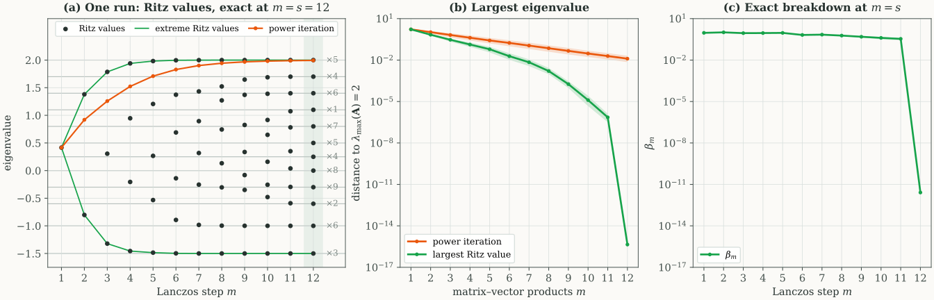
The extreme Ritz values are the extreme Rayleigh quotients over a growing family of subspaces. They can therefore only move outward, toward the extreme eigenvalues of A, and never overshoot them, as the green curves of panel (a) in Figure 6 show.
Proof
Every vector in Km(A,q1) has a unique representation
x=Qmy.
Moreover,
∥x∥2=y⊤Qm⊤Qmy=∥y∥2,
and
x⊤Ax=y⊤Tmy.
Let s1,…,sm be an orthonormal eigenbasis of Tm, with eigenvalues ϑ1,…,ϑm. For any unit vector
y=i=1∑mcisi,i=1∑mci2=1,
we have
y⊤Tmy=i=1∑mϑici2.
Thus
iminϑi≤y⊤Tmy≤imaxϑi.
The lower and upper bounds are attained by eigenvectors associated with the smallest and largest eigenvalues. This proves the two variational identities.
Since Km(A,q1)⊆Km+1(A,q1),
minimizing over the larger set can only decrease the minimum, while maximizing over the larger set can only increase the maximum. Therefore,
ϑmin(m+1)≤ϑmin(m),ϑmax(m)≤ϑmax(m+1).
Finally, every unit vector x∈Rd satisfies
λmin(A)≤x⊤Ax≤λmax(A),
as follows from the same eigenbasis expansion for A. This gives the remaining bounds.
■□
This characterization provides a precise connection with power iteration. Started from v0=q1, and whenever Am−1q1=0, the normalized power iterate
vm−1=∥Am−1q1∥Am−1q1
belongs to Km(A,q1). Consequently,
ϑmin(m)≤vm−1⊤Avm−1≤ϑmax(m).
Lanczos optimizes the Rayleigh quotient over all unit vectors in the available Krylov subspace. The normalized power vector is one particular member of that subspace.
Both estimates cost m matrix–vector products: Tm needs Aq1,…,Aqm, and the Rayleigh quotient of vm−1 needs Av0,…,Avm−1. The eigenvalue of largest magnitude is λmax(A) or λmin(A). In the first case, vm−1⊤Avm−1≤ϑmax(m)≤λmax(A), and in the second, λmin(A)≤ϑmin(m)≤vm−1⊤Avm−1. Either way, at an equal number of products, the extreme Ritz value on the side of the dominant eigenvalue is at least as close to it as the power-iteration estimate (middle panel of the figure in Section 4.9).
This variational statement does not imply that Lanczos has a lower total runtime for every matrix. Constructing and retaining the basis introduces additional work and storage.
4.8 Proposition 3 [Exact termination and the eigenvalues recovered by one run]
For each λ∈Λ(A), let Πλ be the orthogonal projection onto Eλ. Define
Λ1={λ∈Λ(A):Πλq1=0},s=∣Λ1∣.
Here Λ1 contains distinct eigenvalues, irrespective of their multiplicities.
A single Lanczos run terminates at exactly iteration s:
βj>0(1≤j<s),βs=0.
At termination,
AQs=QsTs,
and the eigenvalues of Ts are precisely the elements of Λ1, each appearing once.
Remark 15 [One direction per distinct eigenvalue]
A run can only discover the eigenvalues present in q1, and it discovers each of them once, however large its multiplicity. Inside the Krylov subspace, the whole eigenspace Eλ is represented by the single vector Πλq1. The number of steps before an exact breakdown is therefore the number of distinct eigenvalues present in q1, not d.
Proof
Write
pλ=Πλq1,λ∈Λ1,
and define
W=span{pλ:λ∈Λ1}.
The vectors pλ are nonzero and mutually orthogonal, so
dimW=s.
The Krylov subspaces lie in W. Every power of A applied to q1 belongs to W, because
q1=λ∈Λ1∑pλ
and, for k≥1,
Akq1=λ∈Λ1∑λkpλ.
Therefore,
Km(A,q1)⊆Wfor every m.
The Krylov subspace of order s equals W. For each λ∈Λ1, define the ℓλ is the unique polynomial of degree at most s−1 that equals 1 at λ and 0 at the other s−1 points of Λ1. Applied to A, it keeps the component of q1 along Eλ and removes every other component present in q1.
ℓλ(t)=μ∈Λ1μ=λ∏λ−μt−μ.
When s=1, the empty product is defined as 1. This polynomial has degree at most s−1 and satisfies
ℓλ(μ)={1,0,μ=λ,μ=λ,μ∈Λ1.
Consequently,
ℓλ(A)q1=μ∈Λ1∑ℓλ(μ)pμ=pλ.
Since ℓλ has degree at most s−1,
pλ∈Ks(A,q1).
Thus
W⊆Ks(A,q1),
and hence
Ks(A,q1)=W.
No breakdown before iteration s. Suppose a breakdown occurred at some m<s. Lemma 3 would give
AQm=QmTm,
so
Km(A,q1)=range(Qm)
would be invariant under A. Since it contains q1, it would then contain every power Akq1, and therefore
Ks(A,q1)⊆Km(A,q1).
This is impossible, because
dimKs(A,q1)=s>m=dimKm(A,q1).
Thus no breakdown occurs before iteration s.
Breakdown at iteration s. At iteration s, all columns of Qs belong to W. Since W is spanned by eigenvectors, it is invariant under A. Therefore,
Thus the s vectors yλ form an orthonormal basis of Rs. The corresponding elements of Λ1 are therefore all the eigenvalues of Ts, each appearing once.
■□
4.9 Corollary 3 [Random initialization and repeated eigenvalues]
If g∼N(0,Id) and q1=g/∥g∥, then, with probability one, a terminating Lanczos run recovers every distinct eigenvalue of A. If A has d distinct eigenvalues, the run reaches s=d and yields a complete eigenbasis. If eigenvalues are repeated, a single run yields only one eigenvector from each corresponding eigenspace. With probability one, the eigenvector found in Eλ at termination is the normalized projection of q1 onto Eλ.
Proof
For each λ∈Λ(A), the event Πλg=0 means that g lies in the proper linear subspace Eλ⊥, which has Gaussian probability zero. Since there are finitely many distinct eigenvalues, the For finitely many events, the probability that at least one of them occurs is at most the sum of their probabilities. A finite union of probability-zero events therefore has probability zero. gives
P(∃λ∈Λ(A):Πλg=0)≤λ∈Λ(A)∑P(Πλg=0)=0.
Thus Λ1=Λ(A) with probability one, and Proposition 3 applies.
For any polynomial p, Πλp(A)q1=p(λ)Πλq1. Therefore, the projection of the entire Krylov subspace onto Eλ is contained in span{Πλq1}, which is one-dimensional when Πλq1=0. A single run cannot recover additional independent directions in that eigenspace. At termination, the eigenvectors yλ of Ts from the proof of Proposition 3 lift to the Ritz vectors Qsyλ=uλ, the normalized projections of q1.
When the spectrum is simple and every eigenvalue is present in the initialization, s=d. In this case, Qd is an orthogonal matrix, and
A=QdTdQd⊤.
An orthonormal eigenbasis of Td therefore yields a complete orthonormal eigenbasis of A after multiplication by Qd.
■□
An early exact breakdown does not necessarily mean that a complete eigenbasis of A has been found. It means that the current Krylov subspace has become invariant. For example, when A=cId, every initialization produces a breakdown after one iteration, even though the eigenspace has dimension d.
To recover all eigendirections, the construction can continue with new starting vectors orthogonal to the previously generated basis.
Figure 6. The Lanczos method on a symmetric matrix of size d=60 with random eigenvectors and only s=12 distinct eigenvalues, of multiplicities 1 to 9 (labels on the right of panel a), including the eigenvalue 0 with multiplicity 8. (a) One run: Ritz values at each step m (black dots) against the distinct eigenvalues (grey lines). The extreme Ritz values (green) move outward monotonically (Lemma 5), the power-iteration estimate after the same number of products (orange) stays between them, and at m=s=12 the Ritz values are exactly the 12 distinct eigenvalues, each appearing once (Proposition 3). (b) Distance from λmax(A)=2 of the largest Ritz value (green) and of the power-iteration estimate (orange), at equal numbers of matrix–vector products. (c) The coefficient βm falls from about 0.3 at m=11 to about 10−12 at m=12: the exact breakdown of Proposition 3, up to floating-point error. For every starting vector, the 12 Ritz values at m=12 match the 12 distinct eigenvalues to within 3⋅10−15. Panels (b) and (c) show medians over 200 Gaussian starting vectors, with bands containing the middle half of the runs (the interquartile range), and all runs use full reorthogonalization.
4.10 Proposition 4 [Complete decomposition by continuation with new starting vectors]
Let A∈Rd×d be symmetric. Initialize q0=0, β0=0, and any unit vector q1. Run the Lanczos recurrence for j=1,…,d, with the following rule whenever j<d:
qj+1={rj/βj,any unit vector orthogonal to q1,…,qj,βj>0,βj=0.
At a breakdown, retain βj=0 and all previously generated basis vectors.
Then Qd=[q1,…,qd] is orthogonal,
βd=0,AQd=QdTd,
and
A=QdTdQd⊤.
The matrix Td is symmetric and tridiagonal, with a zero off-diagonal entry at every boundary between runs.
If
Td=ZDZ⊤,Z⊤Z=Id,
with D∈Rd×d the diagonal matrix of the eigenvalues of Td, then
V=QdZ
is a complete orthogonal eigenvector matrix of A:
V⊤V=Id,AV=VD.
Remark 16 [Why continuation completes the basis]
Each run discovers one direction in every eigenspace that its starting vector reaches, then stops at an invariant subspace (Proposition 3). Continuing with a new starting vector in the orthogonal complement, which is invariant as well, lets the next run find the directions that the previous runs could not see.
Proof
At an exact breakdown after iteration j,
AQj=QjTj.
Thus range(Qj) is invariant under A.
Its orthogonal complement is also invariant. Indeed, if Qj⊤x=0, symmetry gives
Qj⊤Ax=(AQj)⊤x=(QjTj)⊤x=TjQj⊤x=0.
A new unit vector in this complement therefore starts another Lanczos run entirely within the complement. Since βj=0, the first recurrence of that run contains no contribution from the preceding block.
Within each run, Lemma 3 ensures orthogonality. Vectors from different runs are orthogonal because they lie in orthogonal invariant subspaces. Each run adds at least one vector, and the construction can continue whenever fewer than d vectors have been obtained. Thus it produces d orthonormal vectors.
At the final iteration, rd is orthogonal to every column of Qd. These columns form a basis of Rd, so
rd=0,βd=0.
Collecting all recurrences, including the zero couplings at block boundaries, gives
AQd=QdTd.
Multiplying on the right by Qd⊤ gives
A=QdTdQd⊤.
Finally,
A(QdZ)=QdTdZ=QdZD,
and
(QdZ)⊤(QdZ)=Z⊤Qd⊤QdZ=Z⊤Z=Id.
Therefore, V=QdZ is a complete orthonormal eigenbasis.
■□
A procedural choice of the new starting vector is
g∼N(0,Id),u=g−Qj(Qj⊤g),qj+1=∥u∥u.
When j<d, a fresh Gaussian draw gives u=0 with probability one.
This continuation retains the entire existing basis. It is different from restarting schemes that discard or compress basis vectors to limit memory use.
4.11 Algorithm 2 [Lanczos with reorthogonalization and residual checks]
For finite computations, the preceding identities require additional care. In particular, the short recurrence does not maintain exact orthogonality in floating-point arithmetic. A direct implementation can reorthogonalize each newly computed residual against the stored basis,
rj←rj−Qj(Qj⊤rj),
repeating the projection when needed before computing βj and normalizing. Such See the discussion of full reorthogonalization in Bai et al., Templates for the Solution of Algebraic Eigenvalue Problems. The projection is carried out with classical or modified Gram–Schmidt, and it is repeated when the norm of the new vector drops below about 1/2 of its previous value, which rarely happens. is a standard part of practical Lanczos implementations (Bai et al., 2000). An implementable procedure for estimating selected eigenpairs is therefore the following.
Fix the operator. Provide a routine computing x↦Ax, and keep everything that defines A fixed throughout the run. For a Hessian ∇θ2f(θ), these are θ and the function f, including the data it is evaluated on.
Initialize the basis. Choose a unit vector q1, and set q0=0 and β0=0.
Extend the basis. Compute the Lanczos recurrence, reorthogonalize the residual, and obtain the next basis vector when its norm is sufficiently large.
Solve the small eigenvalue problem. At selected iterations, assemble Tm and compute its desired eigenpairs Tmyi=ϑiyi.
Check candidates using the original operator. Form xi=Qmyi/∥Qmyi∥, and recompute λi=xi⊤Axi and εi=∥Axi−λixi∥. Accept an approximate eigenpair when εi≤εabs+εrel∥Axi∥, where εabs>0 and εrel≥0 are chosen tolerances.
Stop or continue. Stop when the requested candidates satisfy the tolerance or an iteration limit is reached. If the objective is a complete decomposition, use additional orthogonal starting vectors when a run terminates (Proposition 4).
■□
In exact arithmetic, the inexpensive quantity
βm(yi)m
equals the residual norm (Lemma 4). In floating-point arithmetic, loss of orthogonality and the corrections introduced by reorthogonalization perturb the exact tridiagonal identity. The inexpensive expression can be used to screen candidates, while the residual computed with the original operator supplies the final accuracy check. The normalization by ∥Qmyi∥ in step 5 matters for the same reason: when the computed basis is not exactly orthonormal, Qmyi need not have unit norm, and the inexpensive estimate can then be too optimistic (see the implementation discussion of the Lanczos algorithm in Bai et al., 2000).
A small computed βj indicates an approximate breakdown. It is not an exact proof of invariance or spectral completeness. Likewise, satisfying a residual tolerance certifies an approximate eigenpair, not that no more extreme eigenvalue has been missed.
Each basis-extension step requires one matrix–vector product. If CA denotes its cost, m steps require m such products, with total cost mCA, in addition to any products used for explicit residual checks. Retaining Qm requires O(dm) storage. Full reorthogonalization costs O(dj) operations at iteration j, and therefore
j=1∑mO(dj)=O(dm2)
operations over the run, in addition to solving the projected eigenvalue problems.
When A is available only through products, as in the examples of Section 2, the run never forms A. Nevertheless, a complete decomposition with m=d still requires O(d2) storage for the basis, and full reorthogonalization then costs O(d3) operations. The practical benefit is greatest when the required eigenpairs reach the desired accuracy with m≪d.
Figure 7 below compares the two algorithms on the network Hessian of Figure 5 and on the bipartite graph of Figure 2.
Figure 7.Algorithm 2 (green) against Algorithm 1 (blue), with the same constant threshold 10−10∥A∥ on the residuals for A. (a) The network Hessian of Figure 5: Hessian–vector products used until the j eigenpairs of largest absolute value are certified, medians over 20 starting vectors with bands containing the middle half of the runs. For Algorithm 1, the count runs over stages 1 to j. For Algorithm 2, it is the number of Lanczos steps until the j Ritz pairs of largest absolute value pass the inexpensive test βm∣(yi)m∣≤10−10∥A∥ of Lemma 4, plus one product per pair for the explicit check of step 5, whose residuals were all below 5.4⋅10−10. The eight pairs cost 35 products with Algorithm 2 and about 1,000 with Algorithm 1. (b) The complete eigenbasis of the bipartite graph of Figure 2. The first Lanczos run breaks down at step 41, the number of distinct eigenvalues (Proposition 3), where its 41 Ritz pairs all pass the test. Each of the nine continuation runs of Proposition 4 starts in the eigenspace of 0, orthogonally to the basis built so far, and breaks down after one step. The 50 products, plus 50 explicit checks (green square), give all 50 eigenpairs with residuals below 1.2⋅10−11, against 15,296 products for Algorithm 1 with every stage taken to its limit, as in Figure 3.
5. The Arnoldi method
All the matrices of Section 2 are symmetric, and every proof so far uses the spectral theorem. Many matrices known through their products are not symmetric, and for them three facts of Section 1 fail. First, the eigenvalues of a real matrix can be complex, and then they come in conjugate pairs λ,λˉ. Second, eigenvectors of distinct eigenvalues need not be orthogonal. Third, the eigenvectors need not span the whole space: the matrix [0010] has the double eigenvalue 0, but its only eigenvectors are the multiples of [1,0]⊤.
The Krylov subspace of Definition 1 and the Gram–Schmidt process need no symmetry. The Arnoldi method (Arnoldi, 1951) runs Gram–Schmidt on Km(A,q1) for any square matrix, as the Lanczos method does for a symmetric one, and Saad (1980) developed it into a method for approximating a few eigenvalues of a large nonsymmetric matrix. This section follows the plan of Section 4: examples first, then the method worked by hand, its exact properties, the certificate that replaces Lemma 2, and an implementable procedure.
From here on, A∈Rd×d is any real square matrix, and Λ(A)⊂C is the set of its distinct eigenvalues. For a complex vector y, y∗ is its conjugate transpose and ∥y∥=(y∗y)1/2, which is the Euclidean norm when y is real.
5.1 Nonsymmetric matrices known through their products
Random walks on directed graphs. On a directed graph with d nodes, let Wij≥0 be the weight of the edge from node i to node j, with Wij=0 when there is no such edge. An edge from i to j need not come with an edge from j to i, so W is not symmetric. A random walk steps from node i to node j with probability Pij=Wij/∑kWik, assuming that every node has an outgoing edge. The rows of the transition matrix P=diag(W1)−1W sum to one, P1=1. If (pk)i is the probability that the walker is at node i after k steps, then (pk+1)j=∑i(pk)iPij, that is, pk+1=P⊤pk. A stationary distribution, which one step of the walk leaves unchanged, is therefore an eigenvector of P⊤ with eigenvalue 1, P⊤π=π. It gives the long-run fraction of time that the walker spends at each node, and on the graph of hyperlinks between web pages, with random jumps added, it is the PageRank of Brin and Page (1998). The other eigenvalues of P⊤ say how fast pk approaches π, and complex ones make it oscillate on the way, as Figure 8 below shows. A product with P⊤ costs one pass over the edges, (P⊤x)j=∑iPijxi over the edges i→j.
Convection–diffusion. The operator u↦−u′′+cu′ on [0,1], with u(0)=u(1)=0, describes a quantity that diffuses while a flow of speed c carries it, such as heat or a pollutant in a moving fluid. When c=0, it is the operator u↦−u′′ discretized in Section 2.2, and we discretize it in the same way. The grid points are ti=ih for i=0,…,d+1, with step h=1/(d+1). The unknown xi approximates u(ti) at each of the d interior points, and the boundary conditions set x0=xd+1=0. Replacing the derivatives at ti by the centered differences
u′′(ti)≈h2xi+1−2xi+xi−1,u′(ti)≈2hxi+1−xi−1
gives the matrix defined by
(Ax)i=h22xi−(1+γ)xi−1−(1−γ)xi+1,γ=2ch,
for i∈{1,…,d}. When c=0, this is the symmetric matrix (Ax)i=(2xi−xi−1−xi+1)/h2 of that example. When c=0, it is not symmetric, because its entry Ai,i−1=−(1+γ)/h2 below the diagonal differs from the entry Ai−1,i=−(1−γ)/h2 above it. For 0<γ<1, it is similar to a symmetric matrix. With s=(1+γ)/(1−γ) and S=diag(1,s,s2,…,sd−1), the matrix A=S−1AS is symmetric and tridiagonal, with 2/h2 on its diagonal and −1−γ2/h2 on both neighboring diagonals. The eigenvalues of A are therefore real, equal to (2−21−γ2cos(kπ/(d+1)))/h2 for k=1,…,d. The eigenvectors of A, however, are those of A with entry i multiplied by si−1. They are all concentrated near the end of the grid toward which the flow goes, and they are far from orthogonal. A product costs O(d) operations, as for −u′′.
Jacobians of dynamical systems. A system that evolves by x˙=F(x), for a map F:Rd→Rd, is at rest at a point x⋆ where F(x⋆)=0. A small perturbation y=x−x⋆ then evolves approximately by y˙=Jy, where J is the Jacobian of F at x⋆, with entries Jij=∂Fi(x⋆)/∂xj, because F(x⋆+y)≈Jy to first order. If J has a basis of eigenvectors, Jv=λv, the solution is a combination of the terms eλtv, which decay when the real part of λ is negative and grow when it is positive. The equilibrium is therefore stable when every eigenvalue has a negative real part, and the eigenvalues with the largest real part decide. The matrix J is not symmetric in general. A product with it is a directional derivative, Jx=dεdF(x⋆+εx)ε=0, which forward-mode automatic differentiation computes at the cost of a few evaluations of F. In machine learning, simultaneous gradient steps on the two players of a game, such as the generator and the discriminator of a generative adversarial network, follow such a vector field, and eigenvalues of its Jacobian with large imaginary parts make the iterates circle around an equilibrium rather than approach it (Mescheder et al., 2017). The simplest case is minθmaxϕθϕ, where θ˙=−ϕ and ϕ˙=θ, so that J=[01−10], whose eigenvalues ±i describe a pure rotation.
Figure 8. The random walk on a directed graph used in this section (Section 5.1). (a) The graph: 60 nodes in three groups of 20, teal, gold and pink, arranged in the cycle 1 → 2 → 3 → 1 that the large arrows show. Every node has five outgoing edges, four to random nodes of the next group and one to a random node anywhere else. The 259 edges that end in the next group are drawn in the color of the group they leave, and the other 41 in black (dashed). (b) The transition matrix P, with rows and columns ordered by group and Pij=1/5 for every edge i→j: the edges into the next group fill three colored blocks, and the other edges are the scattered black entries. (c) The probability of each group under the distribution pk=(P⊤)kp0 of the walker, started uniformly on group 1. It circulates through the groups with period three and settles at the stationary values 0.335, 0.331 and 0.334, close to 1/3 (grey, dashed). Between steps 10 and 30, the largest gap to these values shrinks by a factor of 0.80 per step. (d) The eigenvalues of P in the complex plane, all inside the unit circle (grey, dashed). The eigenvalue 1 has the eigenvector 1 for P, and the stationary distribution for P⊤. The pair λ2,λˉ2=0.81e±i119∘ produces the circulation of panel (c), a third of a turn per step damped by the factor 0.81. The other 57 eigenvalues have modulus below 0.45.
The figures of this section use a random walk on a graph with three groups of 20 nodes arranged in a cycle, shown in Figure 8 below. Every node has five outgoing edges, four to random nodes of the next group and one to a random node anywhere else, and the walk follows one of them, chosen uniformly. The walk therefore tends to move from group 1 to group 2, then to group 3, and back to group 1. Started in group 1, its distribution circulates through the groups while it settles (panel c), and the eigenvalues explain how. If P⊤ has a basis of eigenvectors, the distribution expands as
pk=π+cλ2kw+cˉλˉ2kwˉ+⋯=π+2Re(cλ2kw)+⋯,
where P⊤w=λ2w, the number c depends on p0, and the dots stand for the terms of the other eigenvalues. The conjugate terms come from λˉ2, which is also an eigenvalue, with eigenvector wˉ, because P is real. Here λ2=0.81ei119∘ (panel d), so λ2k=0.81kei119∘k: the middle term turns by 119∘, about a third of a turn, at each step, which moves the mass from one group to the next, and it shrinks by the factor 0.81. The other 57 eigenvalues have modulus below 0.45, and their terms die out faster.
Power iteration without symmetry. The iteration vk+1=Avk/∥Avk∥ of Section 3 needs no symmetry. For A=P⊤ started from a distribution, it is the walk itself, rescaled: vk=pk/∥pk∥. When a single real eigenvalue λ1 has the largest modulus, as 1 does here, the expansion above shows that the iterates approach its eigenvector, with an error that shrinks like (∣λ2∣/∣λ1∣)k. Two features of Section 3 are lost. The Rayleigh quotient vk⊤Avk converges at that same rate, not at its square as in Theorem 1, because the error of the iterate is no longer orthogonal to the eigenvector. And the next eigenvalues can form a conjugate pair of equal modulus, which defeats power iteration in the way the opposite eigenvalues of Remark 5 do. Once the eigenvector of 1 is deflated, the pair dominates, and the iterates keep turning in the real plane that carries λ2 and λˉ2, without settling on a direction. Panel (b) of Figure 9 below shows both effects, and the Arnoldi method removes them.
5.2 How the method works
The idea The Arnoldi method runs the Gram–Schmidt process on the Krylov subspace
Km(A,q1)={p(A)q1:p is a polynomial of degree at most m−1},
one matrix–vector product per step, exactly as the Lanczos method does, but for a matrix that need not be symmetric. Without symmetry, no coefficient vanishes for free: each step removes the components of the new vector along all the previous basis vectors. The coefficients fill a small upper Hessenberg matrix, and its eigenvalues, real or complex, approximate eigenvalues of A.
After m−1 products, the Krylov subspace contains every vector p(A)q1 with p of degree at most m−1, whatever A is. To search it, we again need an orthonormal basis q1,…,qm, the columns of Qm, and the coordinates of Aqj in that basis, which form the matrix Hm=Qm⊤AQm with entries hij=qi⊤Aqj. The search itself changes. Without symmetry, the eigenvalues are no longer the extreme values of the Rayleigh quotient, so we look instead for a vector x=Qmy of the subspace and a number ϑ whose residual Ax−ϑx is orthogonal to the subspace. An exact eigenpair satisfies this condition, since its residual is zero. Multiplying the residual by Qm⊤ turns this condition into Hmy=ϑy, an m×m eigenvalue problem. Gram–Schmidt on q1,Aq1,A2q1,… computes the basis and the matrix Hm together, and its first steps, compared with those of Section 4.2, show what symmetry was providing. The colors are those of Section 4.2: a purple coefficient is computed by an inner product at the current step, a green one is the length of the new direction, and a grey one vanishes.
Step 1: Gram–Schmidt on K2(A,q1). The unit vector q1 spans K1(A,q1). The first product gives Aq1, and Gram–Schmidt removes its component h11=q1⊤Aq1 along q1 and divides the rest by its length h21. This is Step 1 of Section 4.2, where these numbers were called α1 and β1:
Aq1=h11q1+h21q2.
Step 2: Gram–Schmidt on K3(A,q1). The second product gives Aq2, which brings the same new direction as A2q1, by the argument of Step 2 of Section 4.2, which used no symmetry. Its component along q1 is where the two methods part. For a symmetric matrix, this component was (Aq1)⊤q2=β1, the length found in Step 1. In general,
q1⊤Aq2=(A⊤q1)⊤q2,
and nothing relates A⊤q1 to the Krylov subspace, so this component is a new number h12, computed by an inner product. Removing it and the component h22=q2⊤Aq2 along q2, then normalizing, gives
Aq2=h12q1+h22q2+h32q3.
Step 3: Gram–Schmidt on K4(A,q1). The third product gives Aq3. In Section 4.2, its component along q1 vanished because q1⊤Aq3=(Aq1)⊤q3=0. Here this component is (A⊤q1)⊤q3, nonzero in general, and all three components have to be computed and removed:
Aq3=h13q1+h23q2+h33q3+h43q4.
Some coefficients still vanish. The vector Aq1 lies in K2(A,q1)=span{q1,q2}, so it has no component along q3, and Aq2, which lies in K3(A,q1), has none along q4. These zeros use only the nesting of the Krylov subspaces, not symmetry. Writing the coefficients of Aqj in column j, as the identity (H3)ij=qi⊤Aqj requires, and doing the same for the Lanczos coefficients, gives
In T3, symmetry made each entry above the diagonal either a length already found (orange) or zero (grey). In H3, these entries are new numbers (purple). The zeros below the first subdiagonal remain in both matrices, because they come from the nesting of Krylov subspaces. A matrix whose entries below the first subdiagonal are zero is called upper Hessenberg.
The general step. At step j, the product Aqj lies in Kj+1(A,q1)=span{q1,…,qj+1}, so it has no component beyond qj+1, while its components along all of q1,…,qj have to be computed and removed:
qjAAqj−h1jq1−⋯−hjjqjrj÷hj+1,jqj+1.
Step j costs one product, j inner products and j vector updates, that is, O(dj) operations besides the product, and every basis vector has to be kept. After m steps, the method has used m products, O(dm2) further operations and O(dm) storage. This is the price of nonsymmetry. It equals the cost of the Lanczos method with full reorthogonalization (Algorithm 2), which subtracts all the components anyway, to protect orthogonality in floating-point arithmetic.
Eigenvalues and eigenvectors from the coefficients. Writing the relations Aqj=∑i=1j+1hijqi for j=1,…,m as the columns of one matrix identity gives
AQm=QmHm+hm+1,mqm+1em⊤,
the analogue of the Lanczos identity, with the same leak through the last basis vector. Every eigenpair (ϑ,y) of Hm, with ∥y∥=1, gives a Ritz pair (ϑ,Qmy), and multiplying the identity by y shows again that the residual of the Ritz pair is the leak, of norm hm+1,m∣ym∣. Since Hm is a real matrix that is not symmetric, its eigenvalues can be complex, in conjugate pairs, which is how the method finds the complex eigenvalues of A.
The polynomial reading of Section 4.2 carries over. Up to the factor h21h32⋯hm+1,m, the vector qm+1 is what remains of Amq1 after removing its orthogonal projection onto Km(A,q1), and the Ritz values at step m are the roots of the monic polynomial πm of degree m that makes ∥π(A)q1∥ smallest (Proposition 5). What changes is the size of ∥π(A)q1∥. If A has a basis of eigenvectors and q1=∑λqλ with Aqλ=λqλ, then π(A)q1=∑λπ(λ)qλ as before, but the vectors qλ are no longer orthogonal, so the norm is no longer (∑λ∣π(λ)∣2∥qλ∥2)1/2. Large components can cancel, and a polynomial can make ∥π(A)q1∥ small without being small at the eigenvalues. The Ritz values can then stay far from every eigenvalue until m is large, and in panel (c) of Figure 9 below they leave the real axis although every eigenvalue is real.
5.3 Definition 3 [Arnoldi recurrence and exact breakdown]
Start with a unit vector q1. At iteration j≥1, compute
If hj+1,j>0, define qj+1=rj/hj+1,j and continue. If hj+1,j=0, stop the run, an exact breakdown as in Definition 2. For m≥1, Hm∈Rm×m is the matrix with entries (Hm)ij=hij for i≤j+1 and (Hm)ij=0 for i>j+1.
■□
The coefficients can equally be computed one at a time: starting from w=Aqj, compute hij=qi⊤w and update w←w−hijqi for i=1,…,j. This is the modified Gram–Schmidt process. Each update leaves the inner products of w with the other basis vectors unchanged, since the basis vectors are orthogonal, so in exact arithmetic both orders give the same numbers. In floating-point arithmetic, the one-at-a-time order loses less orthogonality, and implementations repeat the subtraction when needed, as in Algorithm 2.
5.4 Lemma 6 [Orthogonality and Hessenberg projection]
Before and including the first exact breakdown, the Arnoldi vectors satisfy
qi⊤qj=δij,span{q1,…,qm}=Km(A,q1).
With Qm=[q1,…,qm] and the upper Hessenberg matrix Hm of Definition 3,
AQm=QmHm+rmem⊤,Qm⊤rm=0,Hm=Qm⊤AQm.
If A is symmetric, then Hm is the symmetric tridiagonal matrix Tm of Lemma 3, and the Arnoldi vectors are the Lanczos vectors.
Remark 17 [Where the zeros of the projected matrix come from]
The zeros of Tm have two sources. Those below the first subdiagonal come from the nesting of Krylov subspaces: Aqj lies in Kj+1(A,q1), so it has no component along qj+2,qj+3,…. Those above the first superdiagonal come from symmetry, which turns the component qi⊤Aqj into (Aqi)⊤qj. The Arnoldi method keeps the first source and loses the second. This is why Hm is upper Hessenberg, and why each step removes every previous component.
Proof
Orthogonality. Suppose that q1,…,qj are orthonormal. For each i≤j,
qi⊤rj=qi⊤Aqj−l=1∑jhljqi⊤ql=hij−hij=0.
Thus rj is orthogonal to q1,…,qj, and if hj+1,j>0, normalizing it extends the orthonormal family. Unlike the proof of Lemma 3, this one needs no symmetry, because every component is removed explicitly.
Krylov subspaces. The identity holds at m=1. Suppose that span{q1,…,qj}=Kj(A,q1) and hj+1,j>0. The vector qj+1 is a combination of Aqj and q1,…,qj, all of which lie in Kj+1(A,q1), since qj∈Kj(A,q1) and A maps Kj(A,q1) into Kj+1(A,q1). Hence span{q1,…,qj+1}⊆Kj+1(A,q1). The left-hand side has dimension j+1, because its spanning vectors are orthonormal, and the right-hand side is spanned by j+1 vectors, so the two spaces are equal.
Matrix identity. The definition of rj gives Aqj=∑i=1jhijqi+rj, where rj=hj+1,jqj+1 for j<m. These identities, for j=1,…,m, are the columns of AQm=QmHm+rmem⊤. Multiplying on the left by Qm⊤, and using Qm⊤Qm=Im and Qm⊤rm=0 from the orthogonality part, gives Hm=Qm⊤AQm.
The symmetric case. If A is symmetric, then so is Hm=Qm⊤AQm. Its entries below the first subdiagonal vanish, so by symmetry its entries above the first superdiagonal vanish too, and hj−1,j=hj,j−1. Step j therefore subtracts only hj,j−1qj−1 and hjjqj from Aqj, which is the Lanczos step of Definition 2 with αj=hjj and βj−1=hj,j−1. By induction on j, both methods produce the same vectors and the same coefficients, and Hm=Tm.
■□
5.5 Proposition 5 [Ritz pairs, the minimizing polynomial, and exact termination]
Suppose that the run has reached iteration m, that is, hj+1,j>0 for 1≤j<m.
Ritz pairs. Let Hmy=ϑy with y∈Cm and ∥y∥=1, and let x=Qmy. Then
∥x∥=1,x∗Ax=ϑ,Ax−ϑx=rmym,∥Ax−ϑx∥=hm+1,m∣ym∣.
The minimizing polynomial. The characteristic polynomial πm(t)=det(tIm−Hm) is the unique monic polynomial of degree m that minimizes ∥π(A)q1∥, and
πm(A)q1=h21h32⋯hm,m−1rm.
The Ritz values at step m are the roots of πm.
Exact termination. Let μ be the monic polynomial of smallest degree s such that μ(A)q1=0, called the minimal polynomial of q1. A run reaches iteration s and breaks down there: hj+1,j>0 for j<s, and hs+1,s=0. At termination,
AQs=QsHs,det(tIs−Hs)=μ(t),
so the Ritz values are exactly the roots of μ, and every one of them is an eigenvalue of A. If A has a basis of eigenvectors and q1=∑λ∈Λ(A)qλ with Aqλ=λqλ, then
μ(t)=λ∈Λ1∏(t−λ),Λ1={λ∈Λ(A):qλ=0},s=∣Λ1∣,
as in Proposition 3.
Remark 18 [Ritz values lie in the field of values]
Item 1 says that every Ritz value is the value of x∗Ax at a unit vector. It therefore lies in the field of values
W(A)={x∗Ax:x∈Cd,∥x∥=1},
which also contains every eigenvalue, since x∗Ax=λ for a unit eigenvector x. For a symmetric matrix, W(A) is the interval [λmin(A),λmax(A)], and the Ritz values stay between the extreme eigenvalues (Lemma 5). For a nonsymmetric matrix, W(A) is a convex region of the complex plane that can be much larger than the smallest convex set containing the eigenvalues, and the Ritz values can lie anywhere in it. In panel (c) of Figure 9 below, every eigenvalue is real, but the field of values is an oval around them, and the Ritz values spread over it.
Proof
Ritz pairs. As in the proof of Lemma 4, the orthonormality of the columns of Qm gives ∥x∥2=y∗Qm⊤Qmy=∥y∥2=1, and Lemma 6 gives x∗Ax=y∗Qm⊤AQmy=y∗Hmy=ϑ and
Because Hm is upper Hessenberg, multiplying a vector by Hm moves its last nonzero entry down by at most one position. Hence Hmke1 has nonzero entries only in its first k+1 positions, and its entry in position k+1 is the product h21h32⋯hk+1,k of the subdiagonal entries met on the way. If Akq1=QmHmke1 for some k≤m−1, then the identity of Lemma 6 gives
The last factor is the entry of Hmke1 in position m. It vanishes for k≤m−2 and equals h21h32⋯hm,m−1 for k=m−1, which proves both identities by induction from k=0.
Now let π be a monic polynomial of degree m. Combining the identities term by term gives
π(A)q1=Qmπ(Hm)e1+h21h32⋯hm,m−1rm.
For π=πm, the Cayley–Hamilton theorem gives πm(Hm)=0, hence πm(A)q1=h21⋯hm,m−1rm, which is orthogonal to Km(A,q1) by Lemma 6. For any monic π of degree m, the difference π−πm has degree at most m−1, so (π−πm)(A)q1 lies in Km(A,q1), and Pythagoras’ theorem gives
Equality forces (π−πm)(A)q1=0. The vectors q1,Aq1,…,Am−1q1 span the space Km(A,q1), of dimension m by Lemma 6, so they are linearly independent, and the coefficients of π−πm all vanish: π=πm. Finally, the Ritz values are the eigenvalues of Hm, which are the roots of its characteristic polynomial.
Exact termination. For j<s, no monic polynomial of degree j annihilates q1, by the minimality of s. If the run has reached iteration j<s, item 2 at step j therefore gives
h21h32⋯hj,j−1hj+1,j=∥πj(A)q1∥>0,
hence hj+1,j>0, and the run reaches iteration j+1. Starting from j=1, this shows that the run reaches iteration s. There, the monic polynomial μ of degree s gives ∥μ(A)q1∥=0, so the minimum in item 2 is zero. By uniqueness, πs=μ, and h21⋯hs,s−1hs+1,s=∥μ(A)q1∥=0 forces hs+1,s=0. With rs=0, the identity of Lemma 6 becomes AQs=QsHs. If Hsy=ϑy with y=0, then A(Qsy)=ϑQsy with Qsy=0, so every Ritz value at termination is an eigenvalue of A.
The case of a basis of eigenvectors. If q1=∑λqλ with Aqλ=λqλ, then p(A)q1=∑λ∈Λ1p(λ)qλ for every polynomial p. Nonzero eigenvectors of distinct eigenvalues are linearly independent, so p(A)q1=0 exactly when p(λ)=0 for every λ∈Λ1. The monic polynomial of smallest degree with this property is ∏λ∈Λ1(t−λ), of degree ∣Λ1∣.
■□
Item 2 also proves, for the Lanczos method, the statement of Section 4.2 that the Ritz values are the roots of the minimizing polynomial, since Hm=Tm for a symmetric matrix (Lemma 6). Without a basis of eigenvectors, μ can have repeated roots, and Hs then has them as repeated eigenvalues.
5.6 Lemma 7 [Residual certificate without symmetry]
Suppose that A=VDV−1 for an invertible matrix V∈Cd×d, whose columns are eigenvectors, and a diagonal matrix D, which holds the eigenvalues. Let
Remark 19 [A small residual far from the spectrum]
When A is symmetric, V can be chosen orthogonal, so κ(V)=1 and the lemma is Remark 11. Otherwise κ(V) can be large, and it cannot be dropped. Take
A=[0δ10],x=[10],
with a small δ>0. The eigenvalues are ±δ, the Rayleigh quotient is x⊤Ax=0, and the residual Ax−0⋅x=[0,δ]⊤ has norm δ, whereas the distance from 0 to the spectrum is δ. For δ=10−6, the residual is 10−6 and the distance 10−3, a thousand times larger. The eigenvectors [1,±δ]⊤ are nearly parallel, κ(V)=1/δ=1000, and the lemma holds with equality. What a small residual r=Ax−zx always certifies is that (z,x) is an exact eigenpair of a nearby matrix: (A−rx∗)x=Ax−r=zx, and the perturbation has norm ∥rx∗∥=∥r∥. In the example, A−rx⊤=[0010], whose eigenvalue 0 is double. A perturbation of size δ has moved the eigenvalues by δ, and the eigenvalues of a nonsymmetric matrix can in general move much farther than the size of a perturbation. The set of numbers z with ∥Ax−zx∥<ε for some unit vector x is called the ε-pseudospectrum of A, and for a nonsymmetric matrix it can extend far beyond the points within ε of an eigenvalue (Trefethen and Embree, 2005).
Proof
If z is an eigenvalue, the left-hand side is zero. Otherwise, the diagonal matrix D−zId is invertible, and A−zId=V(D−zId)V−1 gives
x=V(D−zId)−1V−1(Ax−zx).
The largest diagonal entry of (D−zId)−1 in absolute value is 1/minλ∈Λ(A)∣λ−z∣, and it is the norm of this diagonal matrix. Taking norms therefore gives
1=∥x∥≤minλ∈Λ(A)∣λ−z∣∥V∥∥V−1∥∥Ax−zx∥,
which is the claim.
■□
For the convection–diffusion matrix of Section 5.1, A=SAS−1 and A=UDU⊤ with U orthogonal, so V=SU diagonalizes A, with κ(V)=∥S∥∥S−1∥=sd−1. Panel (d) of Figure 9 tests Lemma 2 and Lemma 7 on its Ritz pairs.
Figure 9. The Arnoldi method on the two nonsymmetric matrices of Section 5.1. (a) The random walk of Figure 8, through products with P⊤: its eigenvalues (grey dots), its field of values (grey line, Remark 18), the unit circle (grey, dashed), and the Ritz values of one run at m=5, 10 and 20, colored from light to dark. At m=5, the Ritz values 0.75 and −0.23±0.51i already point to the eigenvalue 1 and to the pair λ2,λˉ2. They are within 6⋅10−4 and 3⋅10−4 of them at m=10, and within 1.1⋅10−8 and 5.7⋅10−7 at m=20, while the other Ritz values lie among the remaining eigenvalues. (b) Distance to an eigenvalue against the number of products, as medians over 200 Gaussian starting vectors, with bands containing the middle half of the runs. The Rayleigh quotient of power iteration on P⊤ (orange) approaches 1 at the rate ∣λ2∣=0.81 per product (grey, dotted), with a median error of 1.2⋅10−3 after 20 products and 1.2⋅10−5 after 40, and power iteration never approaches λ2. After 20 products, the Ritz value nearest to 1 (green) is within 4.4⋅10−9 of it, and the one nearest to λ2 (green, dashed) within 4.4⋅10−7. Both reach rounding level, about 10−15, by 40 products. (c) The convection–diffusion matrix with d=40 and γ=0.2, multiplied by h2. Its eigenvalues are real, between 0.046 and 3.954 (black ticks), and its field of values (grey) is an oval that reaches ±0.40i. The Ritz values of one run at m=10, 20 and 30 (light to dark) are all real at m=10, but 14 of them at m=20 and 24 at m=30 are not, with imaginary parts up to 0.32. (d) Distance from each Ritz value to the spectrum against its residual ∥Ax−ϑx∥, for all the Ritz pairs of steps m=1,…,30 from 5 starting vectors, 2,325 pairs per matrix. For the symmetric matrix of −u′′ (γ=0, blue), every point lies below the diagonal, as Lemma 2 requires, and the largest ratio of distance to residual is 0.49. For convection–diffusion (orange), 311 points lie above the diagonal, with distances up to 5.2 times the residual. Lemma 7 holds, with κ(V)=sd−1=2.7⋅103, but it overestimates every distance by a factor of at least 520. The inexpensive residual hm+1,m∣ym∣ of Proposition 5 agrees with the explicit one to a relative 2⋅10−14.
5.7 Algorithm 3 [Arnoldi with reorthogonalization and residual checks]
The procedure follows Algorithm 2, with three differences: every component is removed, the small eigenvalue problem is not symmetric, and the residual certifies less.
Fix the operator. Provide a routine computing x↦Ax, and keep everything that defines A fixed throughout the run.
Initialize the basis. Choose a unit vector q1, for instance a normalized Gaussian vector.
Extend the basis. At step j, compute w=Aqj, remove its components along q1,…,qj, and repeat the removal once, adding the second coefficients to the first. Store the coefficients in column j of Hm, set hj+1,j=∥w∥, and, when this norm is not negligible, qj+1=w/hj+1,j.
Solve the small eigenvalue problem. At selected steps, compute the eigenpairs Hmyi=ϑiyi, with ∥yi∥=1, by a dense eigensolver for nonsymmetric matrices, and select the wanted ones, for instance those of largest modulus or of largest real part. Nonreal Ritz values come in conjugate pairs, and one member of each pair suffices.
Check candidates using the original operator. Screen each candidate with the inexpensive residual hm+1,m∣(yi)m∣ of Proposition 5. For those that pass, form xi=Qmyi/∥Qmyi∥ and compute λi=xi∗Axi and εi=∥Axi−λixi∥, at the cost of one product for a real xi and two for a complex one, applied to its real and imaginary parts. Accept the pair when εi≤εabs+εrel∥Axi∥.
Stop, continue or restart. Stop when the wanted candidates are accepted or a budget is exhausted. When storing Qm or orthogonalizing against it becomes too expensive, restart as described below.
■□
An accepted pair (λi,xi) is an exact eigenpair of a matrix within εi of A (Remark 19). Whether λi is within εi of an eigenvalue of A depends on the sensitivity of the eigenvalues, such as the factor κ(V) of Lemma 7, which the run does not compute. When the eigenvalue itself must be accurate, for instance when the sign of a real part decides the stability of an equilibrium, the residual should be read together with an estimate of that sensitivity, as discussed by Saad (2011) and by Trefethen and Embree (2005).
Since step j costs O(dj) operations and every basis vector is stored, m cannot grow indefinitely. A restart runs the method again from a new starting vector that combines the wanted Ritz vectors, so that the next Krylov subspace concentrates on them. The implicitly restarted Arnoldi method of Sorensen (1992) restarts without any new product. It applies to Hm a few shifted QR steps, with the unwanted Ritz values as shifts, which amounts to multiplying the starting vector by the polynomial ∏(t−ϑ) over those values, a polynomial filter in the sense of Section 4.1 that damps the unwanted eigencomponents. It then keeps a basis of k<m vectors and extends it again. This is the method of the ARPACK software (Lehoucq, Sorensen and Yang, 1998), on which the sparse eigenvalue routines of several scientific computing environments are built. For a symmetric matrix, the procedure computes, in exact arithmetic, the same vectors and coefficients as the Lanczos method (Lemma 6), at the cost of Algorithm 2.
Lars Mescheder, Sebastian Nowozin, and Andreas Geiger, “The Numerics of GANs”, Advances in Neural Information Processing Systems 30, 2017.
Ch. Müntz, “Solution directe de l’équation séculaire et de quelques problèmes analogues transcendants”, Comptes Rendus de l’Académie des Sciences, Paris, 1913.
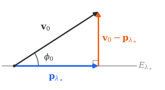 The three vectors form a right triangle: the hypotenuse (black), a side along (blue), and a side perpendicular to it (orange). The angle between a vector and a subspace is the angle between the vector and its orthogonal projection, the smallest angle it makes with a vector of the subspace, so is the angle between and . The tangent is the opposite side over the adjacent side, and since , also and . The hypothesis keeps below ., so that . Then, for every ,