Grokking Beyond the Euclidean Norm of Model Parameters

The Euclidean norm explains some grokking experiments, especially those driven by weight decay, but it is not a universal measure of complexity. The relevant quantity is the property favored late in training.

This post develops the main idea of our ICML 2025 paper, Grokking Beyond the Euclidean Norm of Model Parameters (Notsawo et al., 2025). We will use the memorization time $t_1$ and the generalization time $t_2$ defined in What Is Grokking?.

Paper Pascal Jr Tikeng Notsawo, Guillaume Dumas, and Guillaume Rabusseau, Grokking Beyond the Euclidean Norm of Model Parameters, ICML 2025. arXiv · OpenReview

We demonstrate that grokking can be induced by explicit or implicit regularizationExplicit regularization adds a penalty such as $\beta h(\theta)$ to the objective. Implicit regularization arises from the parameterization, optimizer, initialization, or data even when no corresponding penalty is written in the loss.. More precisely, when there exists a model with a property $P$—for example, sparse or low-rank weights—that generalizes on the problem of interest, gradient descent with a small but non-zero regularization of $P$—for example, $\ell_1$ or nuclear-norm regularization—can result in grokking. This extends previous work showing that small non-zero weight decay induces grokking.

Moreover, our analysis shows that overparameterization through depth can make it possible to grok or ungrok without explicit regularization, which is impossible in the corresponding shallow cases. We further show that the Euclidean norm is not a reliable proxy for generalization when the model is regularized toward another property $P$: in many cases without weight decay, the Euclidean norm grows while the model generalizes anyway. Grokking can also be amplified solely through data selection, with every other hyperparameter fixed.

Why grokking?

We will present two previous explanations related to ours, highlight their limitations, and offer a more general explanation of the phenomenon based on regularization.

Goldilocks zone and LU mechanism

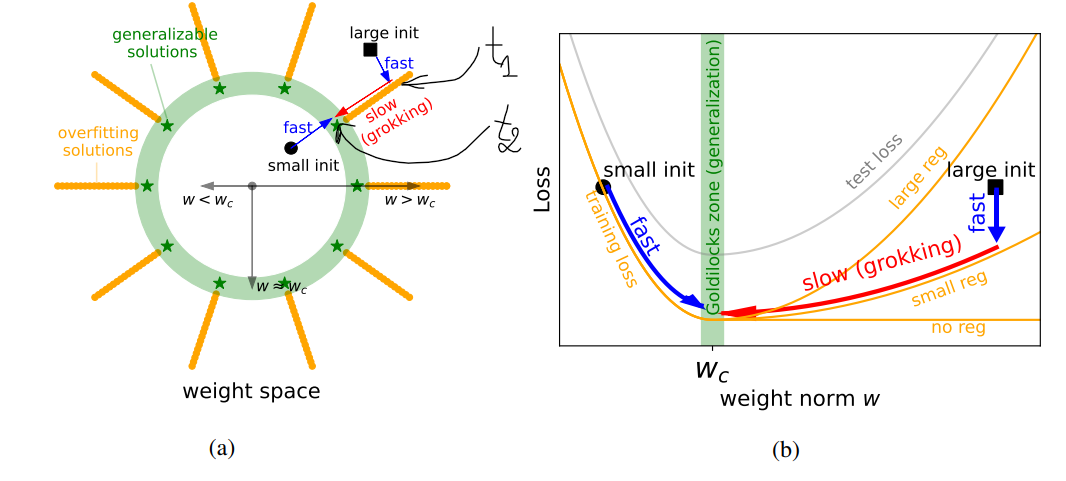
The Goldilocks zoneFort and Scherlis (2018) describe a shell in parameter space where the norm is neither too small to fit nor so large that overfitting dominates—hence “not too small, not too large.” Liu et al. (2023) connect this shell to grokking. (Fort and Scherlis, 2018; Liu et al., 2023) refers to a spherical shell in weight space, at an optimal weight norm $w\approx w_c$, where models achieve good generalization. If $w\ll w_c$, the model underfits and struggles to fit the training data. If $w\gg w_c$, it overfits: training loss is low, but test loss is high.

The LU mechanism of Liu et al. (2023) describes the mismatch between how training and test losses behave as functions of $w$. The training loss forms an L-shape: it decreases quickly and stays near zero for large $w$, because many overfitting solutions exist at high norms. The test loss forms a U-shape: it is minimized near $w_c$ and increases for both smaller and larger norms.

According to this mechanism, the mismatch causes grokking. With a large initialization $w_0 \gg w_c$ and small weight decay $\beta$, the model first overfits at step $t_1$: training loss drops while test loss remains high. It then drifts slowly toward $w_c$ because of weight decay, eventually reaching a point where generalization improves dramatically at step $t_2$.

Why the Euclidean norm cannot be universal

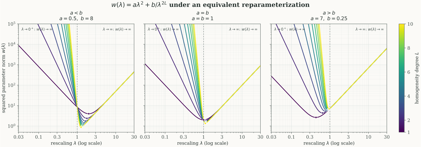
This picture is useful, but a raw parameter norm depends on how we parameterize the same function. Consider $\mathbf y(\mathbf x)=\mathbf B\,\phi(\mathbf A\mathbf x)$ where $\phi$ is positive-$L$-homogeneousThis means that $\phi(\lambda z)=\lambda^L\phi(z)$ for every $z$ and every $\lambda>0$.. ReLU, for instance, is positive-$1$-homogeneous, while the quadratic activations often used for modular arithmetic (Gromov, 2023) are positive-$2$-homogeneous. The reparameterization

$$\mathbf A\longmapsto\lambda\mathbf A, \qquad \mathbf B\longmapsto\lambda^{-L}\mathbf B$$

does not change the predictor, since

$$\frac{\mathbf B}{\lambda^L}\phi(\lambda\mathbf A\mathbf x) = \mathbf B\phi(\mathbf A\mathbf x) \quad \forall \mathbf x.$$

However, using $a:=\|\mathbf A\|_F^2>0$ and $b:=\|\mathbf B\|_F^2>0$, its squared parameter norm becomes $w(\lambda) = a\lambda^2+ \lambda^{-2L} b$. This function decreases until

$$\lambda_0=\left(\frac{Lb}{a}\right)^{\!1/(2L+2)},$$

then increases, with $w(\lambda)\to\infty$ both as $\lambda\to0$ and as $\lambda\to\infty$. Thus, we can arbitrarily increase the norm of the parameters without changing the predictor or its generalization performance. The set of generalizing solutions is therefore not confined to one Euclidean shell around the origin.

There is also a direct experimental objection. We trained the same modular-addition MLP described in What Is Grokking? with a layerwise $\ell_1$, Frobenius, or nuclear normThe entrywise $\ell_1$ norm promotes sparse weights; the Frobenius norm is the Euclidean norm of all entries; the nuclear norm is the sum of singular values and promotes low rank.. Let $\theta$ denote the collection of the model’s weight matrices. The three corresponding norms are

$$\|\theta\|_1=\sum_{\mathbf W\in\theta}\sum_{i,j}|W_{ij}|, \qquad \|\theta\|_2^2=\sum_{\mathbf W\in\theta}\|\mathbf W\|_F^2, \qquad \|\theta\|_*=\sum_{\mathbf W\in\theta}\|\mathbf W\|_*.$$

The first sum is the entrywise $\ell_1$ norm. In each experiment, the model is trained to minimize

$$f(\theta)=g(\theta)+\beta h(\theta),$$

where $g(\theta)$ is the average cross-entropy loss on the training data $\mathcal D_{\mathrm{train}}$, $\beta>0$ is the regularization strength, and $h(\theta)$ is respectively $\|\theta\|_1$, $\|\theta\|_2^2$, or $\|\theta\|_*$. All three induce delayed generalization. Under $\ell_1$ regularization, the Euclidean norm of the full parameter vector can even increase through generalization.

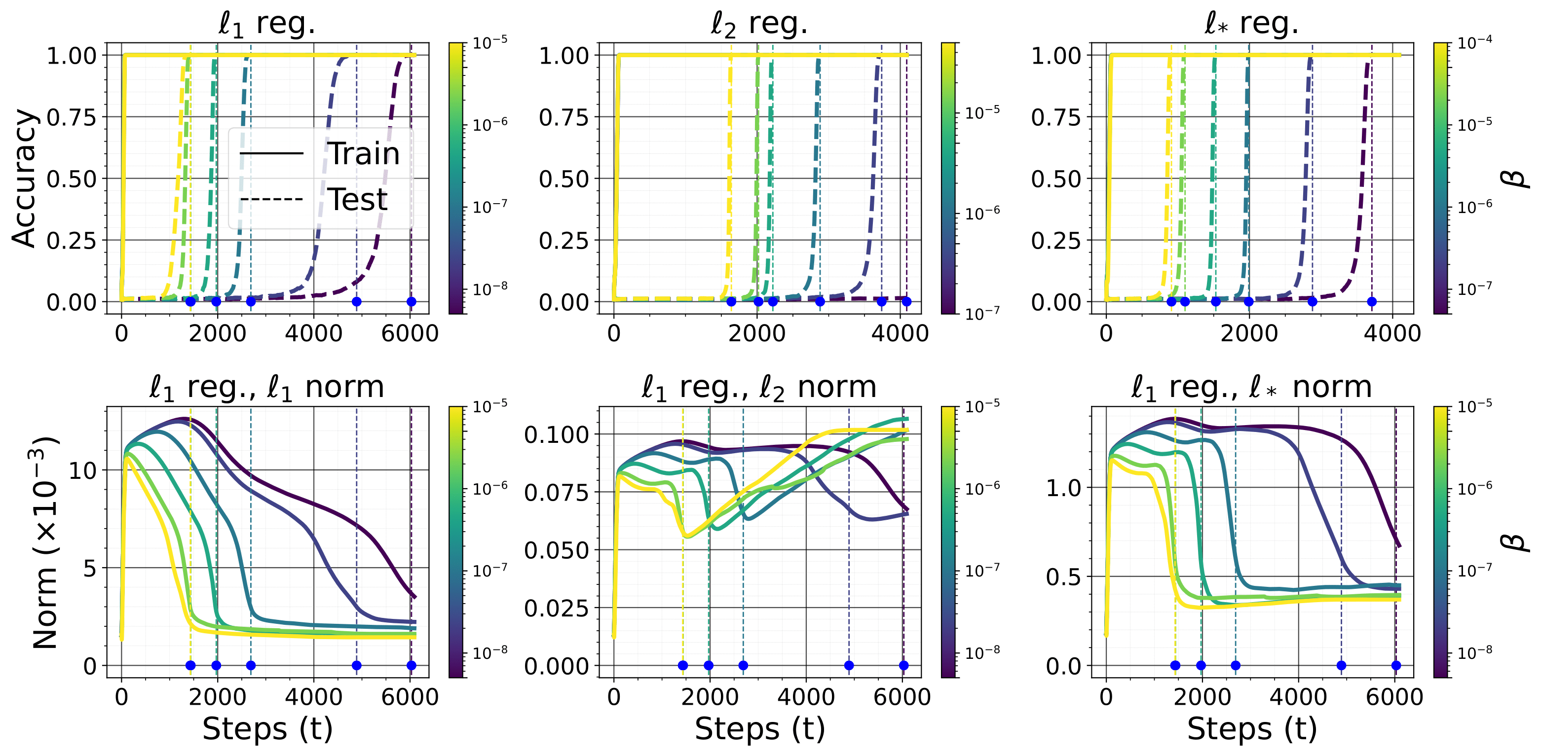
The conclusion is not that the LU picture is useless. It is that the horizontal axis must represent the inductive bias active in the late phaseAn inductive bias is the preference that selects some fitting solutions over others. Here the relevant bias is whichever property the late dynamics continue to improve after the training loss is already small.. Sometimes this is the Euclidean norm; sometimes it is sparsity, low rank, smoothness, or a property induced implicitly by the parameterization.

From the kernel regime to the rich regime

Another explanation describes grokking as a transition from lazy, kernel-like dynamics to a rich regimeIn the kernel regime, parameters move little and the network is well approximated by its linearization at initialization. In the rich regime, features themselves change substantially, allowing behavior unavailable to the fixed linearized model. (Lyu et al., 2023; Kumar et al., 2023). With a sufficiently large initialization, a neural network first behaves approximately like its linearization around initialization. Continued training can eventually leave this kernel regime and enter a rich regime in which the representation changes substantially.

Informal theorem Consider continuous-time gradient flow

$$\frac{d\theta(t)}{dt}=-\nabla_\theta f(\theta(t)), \qquad f(\theta)=g(\theta)+\frac{\beta}{2}\|\theta\|_2^2.$$

Let $\gamma=\|\theta(0)\|_2$ be the initialization scale and set $\tau:=\log(\gamma)/\beta$. Assume that $\beta=\Theta(\gamma^{-c})$ for some fixed $c>0$. Define the NTK featuresThe neural tangent features are the derivatives of the model output with respect to its parameters at initialization. Their inner products define the neural tangent kernel, which governs the linearized training dynamics. at initialization by

$$\mathbf w^{(0)}(\mathbf x) := \left.\nabla_\theta \mathbf y_\theta(\mathbf x)\right|_{\theta=\theta(0)}.$$

Assume that these features are linearly separable in classification, or linearly independent in regression. Also assume that the model is positively $L$-homogeneous in its parametersFor some $L>0$, scaling all parameters by $\lambda>0$ scales the model output by $\lambda^L$: $\mathbf y_{\lambda\theta}(\mathbf x)=\lambda^L\mathbf y_\theta(\mathbf x)$. Bias-free feed-forward networks with homogeneous activations such as ReLU or LeakyReLU satisfy this property; for such networks, $L$ is the number of layers.. Then, as $\gamma\to\infty$, the following holds for every fixed $\epsilon\in(0,1)$.

1. At the early time $t_1=(1-\epsilon)\tau$, the normalized gradient-flow solution points in the direction selected by the linearized NTK problem:

   • In binary classification, it represents the same classifier as the maximum-$\ell_2$-margin classifierAmong separating linear predictors, this solution minimizes $\|\mathbf v\|_2$ under unit-margin constraints. After rescaling, that is equivalent to maximizing the smallest signed distance to the decision boundary. on the NTK features, whose direction is determined by

     $$\underset{\mathbf v}{\operatorname{minimize}} \quad \frac12\|\mathbf v\|_2^2 \qquad\text{subject to}\qquad y\langle\mathbf w^{(0)}(\mathbf x),\mathbf v\rangle\geq1 \quad \forall(\mathbf x,y)\in\mathcal D_{\mathrm{train}}.$$

   • In regression, it follows the minimum-norm interpolating directionWhen many linearized predictors fit every training target exactly, the minimum-norm interpolator selects the one with the smallest Euclidean coefficient norm. in the NTK regime:

     $$\underset{\mathbf v}{\operatorname{minimize}} \quad \frac12\|\mathbf v\|_2^2 \qquad\text{subject to}\qquad \langle\mathbf w^{(0)}(\mathbf x),\mathbf v\rangle=y \quad \forall(\mathbf x,y)\in\mathcal D_{\mathrm{train}}.$$

2. By continuing slightly longer, to $t_2=(1+\epsilon)\tau$, the dynamics leave the NTK regime. The normalized solution approaches the direction of a KKT pointA Karush–Kuhn–Tucker point satisfies stationarity, primal and dual feasibility, and complementary slackness. Under constraint qualifications these conditions are necessary for a constrained local optimum, but in a nonconvex problem they are not sufficient. of the corresponding nonlinear minimum-norm problem

   $$\underset{\theta}{\operatorname{minimize}} \quad \frac12\|\theta\|_2^2$$

   subject to $y\,\mathbf y_\theta(\mathbf x)\geq1$ in binary classification, or $\mathbf y_\theta(\mathbf x)=y$ in regression, for every $(\mathbf x,y)\in\mathcal D_{\mathrm{train}}$.

Here $\epsilon$ is an arbitrary fixed relative separation from the transition time $\tau$. It is not an optimization-error tolerance. The time $t_1$ observes the dynamics an $\epsilon$-fraction before $\tau$, while $t_2$ observes them an $\epsilon$-fraction after $\tau$. A smaller $\epsilon$ places both observations closer to the transition. This is the informal version of the result in Lyu et al. (2023); the original paper gives its precise asymptotic formulation.

Remark Under the usual constraint qualifications, a KKT condition is necessary for a constrained local optimum, and therefore for a global optimum, but it is not generally sufficient—especially when the nonlinear problem is non-convex. KKT points are nevertheless commonly used in theoretical analyses of the implicit bias of gradient methods (Lyu and Li, 2020; Wang et al., 2021; Kunin et al., 2023).

This describes an important change in the dynamics, but the change alone does not imply that the model has learned the intended rule. A late transition generalizes only when the bias of the rich regime is aligned with the target. We will return to this point in “grokking without understanding”.

A property-based mechanism

Let $\mathbf x \in\mathbb R^p$ denote the parameters being optimized. We consider

$$f(\mathbf x)=g(\mathbf x)+\beta h(\mathbf x),$$

where $g:\mathbb R^p\to[0,\infty)$ is the training loss, $h:\mathbb R^p\to[0,\infty)$ measures the favored property, and $\beta>0$ is its strength. We write $\partial h(\mathbf x)$$\partial h(\mathbf x)$ is the set of vectors $\mathbf s$ satisfying $h(\mathbf y)\ge h(\mathbf x)+\langle\mathbf s,\mathbf y-\mathbf x\rangle$ for every $\mathbf y$. It replaces the gradient when a convex penalty is nonsmooth. for the convex subdifferential of $h$ at $\mathbf x$. Subgradient descent with step size $\alpha>0$ gives

$$\mathbf x^{(t+1)} = \mathbf x^{(t)} -\alpha\bigl(G(\mathbf x^{(t)})+\beta H(\mathbf x^{(t)})\bigr), \qquad G=\nabla g, \quad H(\mathbf x^{(t)})\in\partial h(\mathbf x^{(t)}).$$

For small $\beta$, the dynamics have two time scales.

1. Memorization Initially, $G$ dominates $\beta H$. The iterates remain close to $\mathbf x^{(0)}$ and rapidly reduce $g$.
2. Generalization Once $g$ and $G$ are small, the slower term $\beta H$ becomes visible. It moves the solution toward smaller values of $h$ while the training loss remains small.

The paper formalizes the first phase with a local condition. For $r>0$, define

$$B(\mathbf x,r):=\{\mathbf y:\|\mathbf y-\mathbf x\|_2\leq r\},$$

and the Chatterjee–Łojasiewicz constant introduced by Chatterjee (2022)

$$\chi(g,\mathbf x,r) := \inf_{\substack{\mathbf y\in B(\mathbf x,r)\\g(\mathbf y)\neq0}} \frac{\|\nabla g(\mathbf y)\|_2^2}{g(\mathbf y)}.$$

We say that $g$ is $r$-CL at $\mathbf x$ when

$$4g(\mathbf x)<r^2\chi(g,\mathbf x,r).$$

The CL inequality strengthens the classical PL inequalityA PL inequality lower-bounds $\|\nabla g\|_2^2$ by a multiple of the objective gap throughout a region. The local CL condition packages such a gradient-to-loss ratio with enough radius to guarantee that the trajectory stays inside the region where the estimate is useful. (Chatterjee, 2022). PL-type inequalities have been shown to hold for wide overparameterized neural networks in a neighbourhood of their initialization (Liu et al., 2021). The advantage here is that we require the CL inequality only at initialization, whereas standard convergence results under the PL condition assume it over an entire region or domain (Karimi et al., 2020).

This condition only concerns a neighbourhood of the initialization. Under the regularity assumptions in Theorem 2.1 of the paper, if $g$ is $r$-CL at $\mathbf x^{(0)}$, then sufficiently small $\alpha$ and $\beta$ produce the two phases above. For some constant $C>0$, the first reaches $g(\mathbf x^{(t_1)})\leq\epsilon_g$ for any attainable precision $\epsilon_g=\Omega(\beta^C)$Here $\epsilon_g=\Omega(\beta^C)$ means that the requested precision is not asymptotically smaller than a constant multiple of $\beta^C$ as $\beta\to0$. The theorem guarantees every tolerance above that floor., while staying in $B(\mathbf x^{(0)},r)$. For fixed tolerance and distance to the solution set, the sufficient late-phase horizon contains the factor $1/(\alpha\beta)$.

Theorem 2.1 The following is the main two-phase theorem of Notsawo et al. (2025). Take $\mathbf x^{(0)}\in\mathbb R^p$ with

$$g^{(0)}:=g(\mathbf x^{(0)})>0,$$

and assume that $g$ is $r$-CL at $\mathbf x^{(0)}$ for some $r>0$. Write

$$\chi:=\chi(g,\mathbf x^{(0)},r), \qquad 4g^{(0)}<r^2\chi.$$

Assume that $g$ is twice continuously differentiable on a neighbourhood of $B(\mathbf x^{(0)},2r)$ and that the subgradients of $h$ are bounded on $B(\mathbf x^{(0)},r)$. Then there exist $\alpha_{\max},\beta_{\max}>0$ such that, for every $\alpha\in(0,\alpha_{\max})$, one can choose constants $C,D>0$ for which the following statements hold for every $\beta\in(0,\beta_{\max})$.

1. Fast phase. For any attainable precision

   $$\epsilon_g\geq D\beta^C,$$

   there is a $\delta\in(0,1)$ with $\delta=\Theta(\alpha\chi)$ such that one may take

   $$t_1 = \left\lceil \max\left\{ 0, \frac{\log(\epsilon_g/g^{(0)})}{\log(1-\delta)} \right\} \right\rceil$$

   When $\epsilon_g<g^{(0)}$, this choice is $\mathcal O\!\left((\alpha\chi)^{-1}\log(g^{(0)}/\epsilon_g)\right)$, and it satisfies

   $$g(\mathbf x^{(t_1)})\leq\epsilon_g, \qquad \|G(\mathbf x^{(t_1)})\|_2^2=\mathcal O(\epsilon_g), \qquad \mathbf x^{(t)}\in B(\mathbf x^{(0)},r) \quad\forall t\leq t_1.$$

2. Late phase. Define

   $$\Theta_f:=\operatorname*{argmin}_{\mathbf x}f(\mathbf x), \qquad f^*:=\inf_{\mathbf x}f(\mathbf x),$$

   and assume that $\Theta_f$ is nonempty. Let

   $$\operatorname{dist}(\mathbf x,\Theta_f) := \inf_{\mathbf u\in\Theta_f}\|\mathbf x-\mathbf u\|_2,$$

   and let

   $$F(\mathbf x^{(t)}) := G(\mathbf x^{(t)})+\beta H(\mathbf x^{(t)}).$$

   Suppose that, for $t_1\leq t<t_2$,

   $$f(\mathbf u) \geq f(\mathbf x^{(t)}) +\left\langle F(\mathbf x^{(t)}),\mathbf u-\mathbf x^{(t)}\right\rangle \qquad \forall\mathbf u\in\mathbb R^p, \tag{S}$$

   and, for a constant $C'>0$ independent of $t$, $\alpha$, and $\beta$,

   $$\|F(\mathbf x^{(t)})\|_2^2\leq C'\beta^2. \tag{B}$$

   Convexity of $g$ and $h$ is sufficient for (S). For every $\eta>0$, the observation horizon

   $$t_2-t_1 \geq \frac{\operatorname{dist}^2(\mathbf x^{(t_1)},\Theta_f)} {\alpha\beta\eta} \tag{H}$$

   is sufficient to guarantee

   $$\min_{t_1\leq t<t_2} \bigl(f(\mathbf x^{(t)})-f^*\bigr) \leq \frac{\beta}{2}\bigl(\eta+C'\alpha\beta\bigr). \tag{F}$$

   If $g^*:=\inf_{\mathbf x}g(\mathbf x)=0$, define

   $$\Theta_g:=\{\mathbf x:g(\mathbf x)=0\}, \qquad h_g^*:=\inf_{\mathbf x\in\Theta_g}h(\mathbf x).$$

   When $\Theta_f\cap\Theta_g\neq\varnothing$, the same interval contains an iterate satisfying

   $$h(\mathbf x^{(t)})-h_g^* \leq \frac12\bigl(\eta+C'\alpha\beta\bigr). \tag{P}$$

The first item formalizes memorization: for sufficiently small $\beta$, the iterates stay near initialization and minimize $g$ geometrically down to any precision above the $D\beta^C$ floor. If $\beta$ is too large, regularization may intervene before $g$ reaches a smaller precision. In the second phase, once $G$ is of the same order as $\beta H$, the regularizer drives the iterates toward small values of $f$ and $h$. The sufficient delay is of order $1/(\alpha\beta)$. The factor $\alpha$ is absent from the continuous-time result of Lyu et al. (2023) because their dynamics are parameterized directly by time.

The bounds are for the best iterate in the interval. Condition (H) is a sufficient observation horizon; it is not asserted to be the exact first-crossing time.

Complete proof of Theorem 2.1

Show the complete five-step proof

We now prove both phases under the local assumptions above. The descent estimate used in the first phase is the second-order Taylor estimate from the report, equivalently the local descent lemma proved in Smoothness, Descent, and Cocoercivity.

Choice of the local constants

Set

$$M_g := \sup_{\mathbf x\in B(\mathbf x^{(0)},r)}\|G(\mathbf x)\|_2, \qquad M_h := \sup_{\mathbf x\in B(\mathbf x^{(0)},r)} \sup_{H\in\partial h(\mathbf x)}\|H\|_2,$$

and

$$L := \sup_{\mathbf x\in B(\mathbf x^{(0)},2r)} \|\nabla^2g(\mathbf x)\|_{2\to2}.$$

These quantities are finite by the assumptionsThe closed finite-dimensional balls are compact. Continuity of $G$ and $\nabla^2g$ makes their norms attain finite maxima there, while boundedness of the subgradients of $h$ is assumed explicitly.. Because $4g^{(0)}<r^2\chi$, we can choose $\varepsilon_0\in(0,1)$ and $\kappa\in(0,\varepsilon_0)$ such that

$$4g^{(0)} < \left(\frac{1-\varepsilon_0}{1+\kappa}\right)^2r^2\chi. \tag{1}$$

Choose $\beta_{\max}>0$ so that

$$\beta_{\max}M_h \leq \kappa\|G(\mathbf x^{(0)})\|_2, \tag{2}$$

and choose $\alpha>0$ small enough that

$$\alpha < \min\left\{ \frac{r}{M_g+\beta_{\max}M_h}, \frac{2(\varepsilon_0-\kappa)}{L(1+\kappa)^2}, \frac{1}{L(1+\kappa)}, \frac{1}{(1-\varepsilon_0)\chi} \right\}. \tag{3}$$

Finally, define

$$\delta:=(1-\varepsilon_0)\alpha\chi\in(0,1), \qquad q:=1-\alpha L(1+\kappa)\in(0,1). \tag{4}$$

The symbols $\varepsilon_0$ and $\kappa$ are local proof parameters; they are unrelated to the $\epsilon$ used in the preceding kernel-to-rich theorem.

Step 1: geometric decay while the loss gradient dominates

For brevity, write

$$g_t:=g(\mathbf x^{(t)}), \qquad G_t:=G(\mathbf x^{(t)}), \qquad H_t:=H(\mathbf x^{(t)}), \qquad F_t:=G_t+\beta H_t.$$

Suppose that $\mathbf x^{(t)}\in B(\mathbf x^{(0)},r)$ and that

$$\beta\|H_t\|_2\leq\kappa\|G_t\|_2. \tag{5}$$

The first condition in (3) ensures that the segment from $\mathbf x^{(t)}$ to $\mathbf x^{(t+1)}$ remains in $B(\mathbf x^{(0)},2r)$. On that segment, $g$ is $L$-smooth. Applying the descent lemma and then adding and subtracting the regularization contribution gives

$$\begin{aligned} g_{t+1} &\leq g_t-\alpha\langle G_t,F_t\rangle +\frac{L\alpha^2}{2}\|F_t\|_2^2\\ &= g_t-\alpha\|G_t\|_2^2 -\color{#a55a65}{\alpha\beta\langle G_t,H_t\rangle} +\frac{L\alpha^2}{2}\|G_t+\beta H_t\|_2^2\\ &\leq g_t-\alpha\left[ 1-\kappa-\frac{L\alpha}{2}(1+\kappa)^2 \right]\|G_t\|_2^2\\ &\leq g_t-(1-\varepsilon_0)\alpha\|G_t\|_2^2. \end{aligned} \tag{6}$$

The penultimate line uses (5), Cauchy–Schwarz, and $\|F_t\|_2\leq(1+\kappa)\|G_t\|_2$; the last line follows from (3). Because $\mathbf x^{(t)}$ lies in the CL ball,

$$\|G_t\|_2^2\geq\chi g_t.$$

Consequently,

$$g_{t+1} \leq (1-\delta)g_t, \qquad g_t-g_{t+1} \geq \frac{\delta}{\chi}\|G_t\|_2^2. \tag{7}$$

As long as (5) holds, iterating the first inequality yields

$$g_t\leq(1-\delta)^t g^{(0)}. \tag{8}$$

Step 2: the iterates remain in the CL neighbourhood

Assume that (5) holds for $t=j,\ldots,k-1$. From (7),

$$\begin{aligned} \sum_{t=j}^{k-1}\alpha\|F_t\|_2 &\leq \alpha(1+\kappa)\sum_{t=j}^{k-1}\|G_t\|_2\\ &\leq \alpha(1+\kappa)\sqrt{\frac{\chi}{\delta}} \sum_{t=j}^{k-1}\sqrt{g_t-g_{t+1}}. \end{aligned} \tag{9}$$

To bound the last sum, factor each difference and use Cauchy–Schwarz:

$$\begin{aligned} \sum_{t=j}^{k-1}\sqrt{g_t-g_{t+1}} &= \sum_{t=j}^{k-1} \sqrt{\bigl(\sqrt{g_t}-\sqrt{g_{t+1}}\bigr) \bigl(\sqrt{g_t}+\sqrt{g_{t+1}}\bigr)}\\ &\leq \left[ \bigl(\sqrt{g_j}-\sqrt{g_k}\bigr) \sum_{t=j}^{k-1} \bigl(\sqrt{g_t}+\sqrt{g_{t+1}}\bigr) \right]^{1/2}\\ &\leq 2\sqrt{\frac{g^{(0)}}{\delta}} (1-\delta)^{j/2}. \end{aligned} \tag{10}$$

For the last inequality, we used (8) and

$$\sum_{t=j}^{\infty}(1-\delta)^{t/2} = \frac{(1-\delta)^{j/2}}{1-\sqrt{1-\delta}} \leq \frac{2(1-\delta)^{j/2}}{\delta}.$$

Combining (9) and (10), and using the definition of $\delta$, gives

$$\sum_{t=j}^{k-1}\alpha\|F_t\|_2 \leq (1-\delta)^{j/2} \sqrt{ \frac{4(1+\kappa)^2g^{(0)}} {\chi(1-\varepsilon_0)^2} }. \tag{11}$$

At $j=0$, the right-hand side is strictly smaller than $r$ by (1). Since

$$\|\mathbf x^{(k)}-\mathbf x^{(0)}\|_2 \leq \sum_{t=0}^{k-1}\alpha\|F_t\|_2,$$

we obtain $\mathbf x^{(k)}\in B(\mathbf x^{(0)},r)$. This proves inductively that every iterate remains in the CL ball for as long as the dominance condition (5) holds.

Step 3: the dominance condition lasts long enough

While (5) holds, local $L$-smoothness and the update give

$$\begin{aligned} \|G_{t+1}\|_2 &\geq \|G_t\|_2-\|G_{t+1}-G_t\|_2\\ &\geq \|G_t\|_2-L\|\mathbf x^{(t+1)}-\mathbf x^{(t)}\|_2\\ &\geq \bigl(1-\alpha L(1+\kappa)\bigr)\|G_t\|_2\\ &=q\|G_t\|_2. \end{aligned} \tag{12}$$

Fix an integer $k\geq0$. If

$$\kappa\|G_0\|_2 \geq q^{-k}\beta M_h, \tag{13}$$

then an induction using (12) gives, for every $0\leq t\leq k$,

$$\|G_t\|_2 \geq q^t\|G_0\|_2 \geq \frac{\beta M_h}{\kappa q^{k-t}}.$$

Hence

$$\beta\|H_t\|_2 \leq \beta M_h \leq \kappa\|G_t\|_2.$$

Thus (13) guarantees the dominance condition, the geometric loss decay, and containment in the CL ball through step $k$.

Step 4: reaching every precision above the $\beta^C$ floor

For $0<\epsilon_g<g^{(0)}$, define

$$t_1 := \left\lceil \frac{\log(\epsilon_g/g^{(0)})} {\log(1-\delta)} \right\rceil;$$

take $t_1=0$ when $\epsilon_g\geq g^{(0)}$. Equation (8) gives $g_{t_1}\leq\epsilon_g$. It remains to ensure that (13) is valid up to this step.

Define

$$C := \frac{\log(1-\delta)}{\log q}>0, \qquad D := g^{(0)} \left( \frac{M_h}{\kappa q\|G_0\|_2} \right)^C. \tag{14}$$

If $\epsilon_g\geq D\beta^C$, then $t_1$ satisfies (13). Indeed, $t_1$ is at most one plus its unrounded value, and (14) is exactly the rearrangement of

$$\beta M_hq^{-t_1} \leq \kappa\|G_0\|_2.$$

Therefore $\mathbf x^{(t)}\in B(\mathbf x^{(0)},r)$ for every $t\leq t_1$, and $g_{t_1}\leq\epsilon_g$. Finally, (6) and the nonnegativity of $g$ imply

$$(1-\varepsilon_0)\alpha\|G_{t_1}\|_2^2 \leq g_{t_1}-g_{t_1+1} \leq g_{t_1}.$$

Thus

$$\|G_{t_1}\|_2^2 \leq \frac{\epsilon_g}{(1-\varepsilon_0)\alpha} = \mathcal O(\epsilon_g),$$

which completes the proof of the fast phase.

Step 5: the late-phase distance argument

Take any $\mathbf x^*\in\Theta_f$. From (S),

$$\langle F_t,\mathbf x^{(t)}-\mathbf x^*\rangle \geq f(\mathbf x^{(t)})-f^*. \tag{15}$$

Using the update $\mathbf x^{(t+1)}=\mathbf x^{(t)}-\alpha F_t$ and then (15), we obtain

$$\begin{aligned} \|\mathbf x^{(t+1)}-\mathbf x^*\|_2^2 &= \|\mathbf x^{(t)}-\mathbf x^*\|_2^2 -2\alpha\langle F_t,\mathbf x^{(t)}-\mathbf x^*\rangle +\alpha^2\|F_t\|_2^2\\ &\leq \|\mathbf x^{(t)}-\mathbf x^*\|_2^2 -2\alpha\bigl(f(\mathbf x^{(t)})-f^*\bigr) +\alpha^2\|F_t\|_2^2. \end{aligned} \tag{16}$$

Sum (16) from $t=t_1$ to $t_2-1$. The squared-distance terms telescope, so dropping the final nonnegative distance gives

$$2\alpha \sum_{t=t_1}^{t_2-1} \bigl(f(\mathbf x^{(t)})-f^*\bigr) \leq \|\mathbf x^{(t_1)}-\mathbf x^*\|_2^2 +\alpha^2 \sum_{t=t_1}^{t_2-1}\|F_t\|_2^2.$$

Divide by $2\alpha(t_2-t_1)$, bound the minimum by the average, and minimize over $\mathbf x^*\in\Theta_f$:

$$\min_{t_1\leq t<t_2} \bigl(f(\mathbf x^{(t)})-f^*\bigr) \leq \frac{\operatorname{dist}^2(\mathbf x^{(t_1)},\Theta_f)} {2\alpha(t_2-t_1)} + \frac{\alpha}{2} \max_{t_1\leq t<t_2}\|F_t\|_2^2. \tag{17}$$

By (B) and (H),

$$\frac{\operatorname{dist}^2(\mathbf x^{(t_1)},\Theta_f)} {2\alpha(t_2-t_1)} \leq \frac{\beta\eta}{2}, \qquad \frac{\alpha}{2}\max_{t_1\leq t<t_2}\|F_t\|_2^2 \leq \frac{C'\alpha\beta^2}{2}.$$

Substitution into (17) proves (F).

Finally, suppose $\Theta_f\cap\Theta_g\neq\varnothing$. Then $f^*=\beta h_g^*$; otherwise a zero-loss point with smaller $h$ would contradict optimality in $\Theta_f$. Since $g\geq0$,

$$\beta\bigl(h(\mathbf x^{(t)})-h_g^*\bigr) \leq f(\mathbf x^{(t)})-f^*.$$

Taking the minimum over the interval and dividing (F) by $\beta$ proves (P). This completes the proof.

Sparse recovery: the ℓ₁ bias

Let $\mathbf a^*\in\mathbb R^n$ be a sparse vector and suppose that we observe

$$\mathbf y^*=\mathbf X\mathbf a^*+\boldsymbol\xi, \qquad \mathbf X\in\mathbb R^{N\times n},$$

where $\mathbf y^*,\boldsymbol\xi\in\mathbb R^N$ and $\boldsymbol\xi$ is measurement noise. We optimize the coefficients $\mathbf a\in\mathbb R^n$ using

$$f(\mathbf a) = \frac12\|\mathbf X\mathbf a-\mathbf y^*\|_2^2 +\beta\|\mathbf a\|_1.$$

This is the sparse-recovery specialization studied in Theorems 3.1 and 3.3 of Notsawo et al. (2025). The ideal formulation minimizes $\|\mathbf a\|_0$, the number of non-zero coefficients, subject to fitting the measurements within the noise tolerance. That problem is NP-hard (Natarajan, 1995), so $\|\mathbf a\|_0$ is replaced by $\|\mathbf a\|_1$$\ell_0$ directly counts nonzero entries but is combinatorial and nonconvex. $\ell_1$ is its tightest convex, positively homogeneous surrogate and can recover the same sparse solution under suitable measurement conditions. (Donoho, 2006; Chandrasekaran et al., 2012). See Foucart and Rauhut (2013) for a systematic treatment of compressed sensing.

With the near-zero initialization used in our experiment, the early, data-fit-dominated phase moves toward the minimum-Euclidean-norm least-squares solutionThe Moore–Penrose pseudoinverse selects, among all least-squares solutions, the one orthogonal to the null space of $\mathbf X$—equivalently, the solution with the smallest Euclidean norm.

$$\widehat{\mathbf a} := (\mathbf X^\top\mathbf X)^\dagger\mathbf X^\top\mathbf y^*.$$

This solution minimizes the measurement residual and, when $\mathbf y^*$ lies in the range of $\mathbf X$, fits the measurements. In an underdetermined problem it need not equal the sparse target. After memorization, the $\ell_1$ subgradient dominates and pushes the iterates toward a sparse fitting solution.

Definition A matrix $\mathbf X\in\mathbb R^{N\times n}$ satisfies the robust null-space propertyNo vector that is nearly invisible to $\mathbf X$ may concentrate most of its $\ell_1$ mass on the target support $S$. This prevents an alternative sparse vector from fitting almost the same measurements. with constants $\rho\in(0,1)$ and $\tau>0$ relative to a set $S\subset[n]$ when

$$\|\mathbf u_S\|_1 \leq \rho\|\mathbf u_{S^c}\|_1 +\tau\|\mathbf X\mathbf u\|_2 \qquad\text{for every }\mathbf u\in\mathbb R^n.$$

Recovery theorem If $\mathbf X$ satisfies this property relative to the support of $\mathbf a^*$, then, under the learning-rate, regularization, and noise conditions of Notsawo et al. (2025), there exist constants $C_1,C_2,C_3>0$ such that the best iterate in the late phase satisfies

$$\|\mathbf a^{(t)}-\mathbf a^*\|_1 \leq C_1\eta+C_2\alpha\beta+C_3\|\boldsymbol\xi\|_2$$

once $t_2-t_1\geq\|\mathbf a^{(t_1)}-\mathbf a^*\|_2^2/(\alpha\beta\eta)$.

When $\mathbf X$ contains enough information for $\mathbf a^*$ to be the stable minimum-$\ell_1$ fit, the recovery theorems give a best-iterate $\ell_1$ recovery error of order $\eta+\alpha\beta+\|\boldsymbol\xi\|_2$ once the late-phase horizon is of order

$$\frac{\|\mathbf a^{(t_1)}-\mathbf a^*\|_2^2} {\alpha\beta\eta}.$$

In the noiseless scaling experiment, let $t_{\mathrm{plat}}$ denote the selected plateau checkpointWe choose the first pair of recorded recovery errors lying within $5\%$ of the mean of the final three. If no such pair exists, we use the final checkpoint.. We observe

$$\|\mathbf a^{(t_{\mathrm{plat}})}-\mathbf a^*\|_1 \propto\alpha\beta, \qquad t_{\mathrm{plat}} \propto \frac{\|\widehat{\mathbf a}-\mathbf a^*\|_\infty}{\alpha\beta}.$$

This is grokking in a recovery problem. A small residual $\|\mathbf X\mathbf a^{(t)}-\mathbf y^*\|_2$ marks memorization; a small recovery error $\|\mathbf a^{(t)}-\mathbf a^*\|_2$ marks generalization.

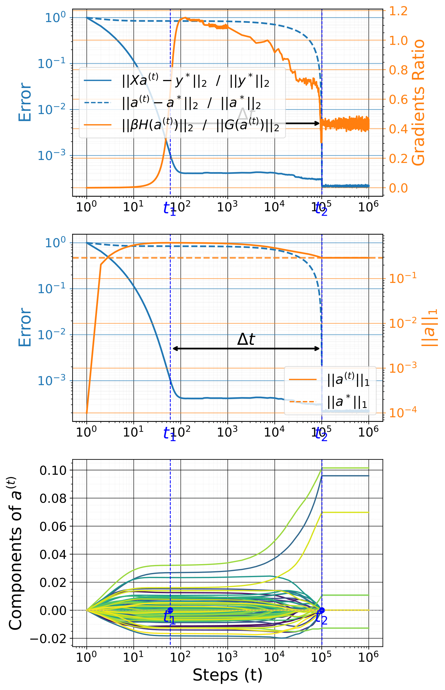
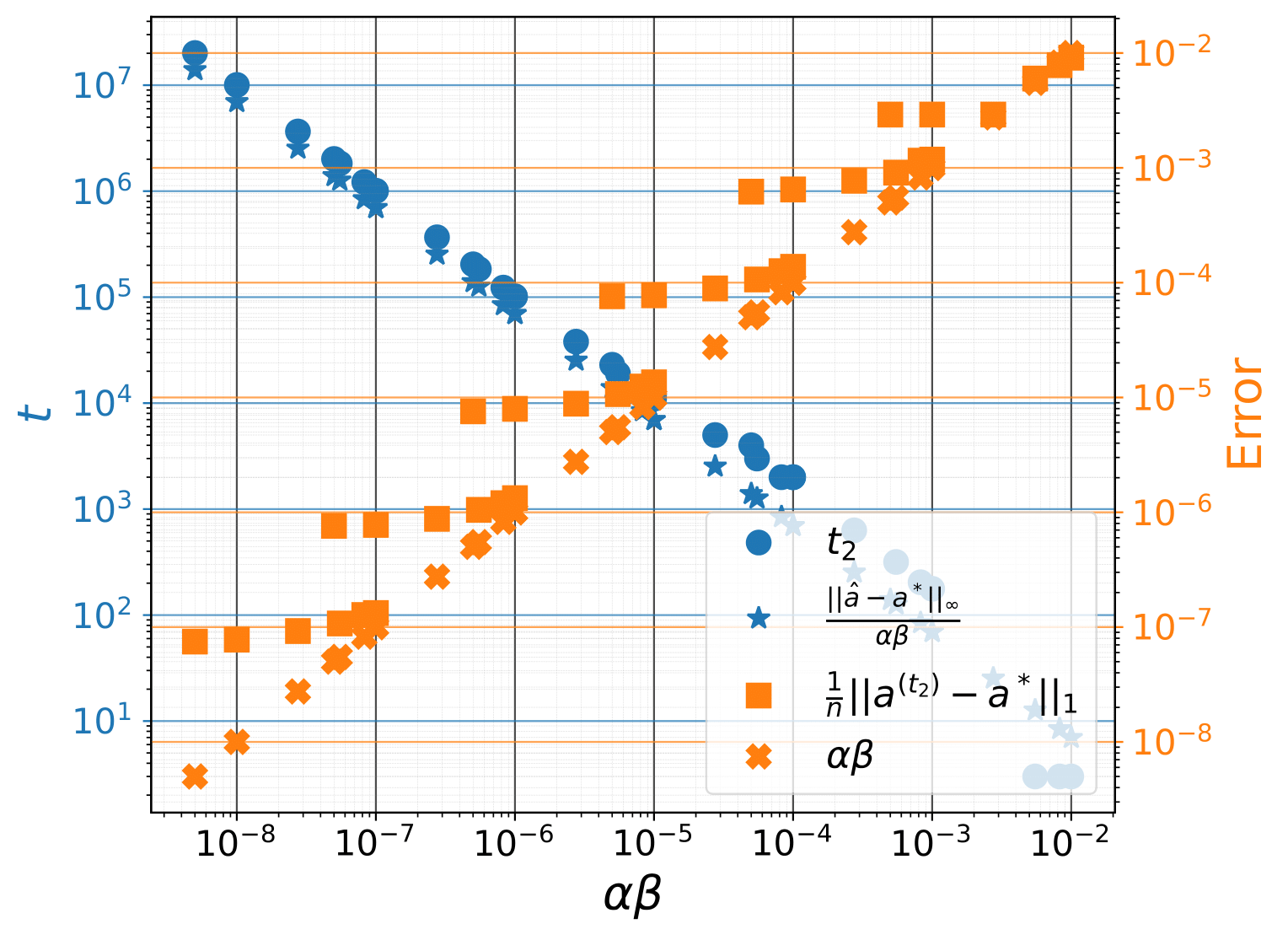
Small $\alpha\beta$ therefore lowers the observed recovery error, but makes the generalization phase longer. This is the same tradeoff predicted by the generic theorem.

Low-rank recovery: the nuclear norm

The matrix analogue replaces sparsity by low rank. Let $\mathbf A^*\in\mathbb R^{n_1\times n_2}$ have rank much smaller than $\min(n_1,n_2)$, and observe

$$\mathbf y^*=\mathbf X\operatorname{vec}(\mathbf A^*)+\boldsymbol\xi, \qquad \mathbf y^*,\boldsymbol\xi\in\mathbb R^N.$$

Here $\operatorname{vec}(\mathbf A)$$\operatorname{vec}(\mathbf A)$ stacks the columns of $\mathbf A$ one beneath another to form a vector in $\mathbb R^{n_1n_2}$. and $\mathbf X\in\mathbb R^{N\times n_1n_2}$ is the measurement matrix. We optimize the matrix $\mathbf A$ through

$$f(\mathbf A) = \frac12\|\mathbf X\operatorname{vec}(\mathbf A)-\mathbf y^*\|_2^2 +\beta\|\mathbf A\|_*,$$

where $\|\mathbf A\|_*=\sum_i\sigma_i(\mathbf A)$ is the nuclear normThe nuclear norm sums the singular values. It is the matrix analogue of the $\ell_1$ norm and is the standard convex surrogate for rank.. If

$$\operatorname{vec}(\widehat{\mathbf A}) := (\mathbf X^\top\mathbf X)^\dagger\mathbf X^\top\mathbf y^*,$$

then, from the near-zero initialization used in our experiment, the early phase approaches the least-squares fit $\widehat{\mathbf A}$, while the late nuclear-norm dynamics favor a low-rank solution. Under the recovery conditions in the paper, a best iterate has nuclear-norm recovery error of order $\eta+\alpha\beta+\|\boldsymbol\xi\|_2$ once the late-phase horizon is of order

$$\frac{\|\mathbf A^{(t_1)}-\mathbf A^*\|_F^2} {\alpha\beta\eta}.$$

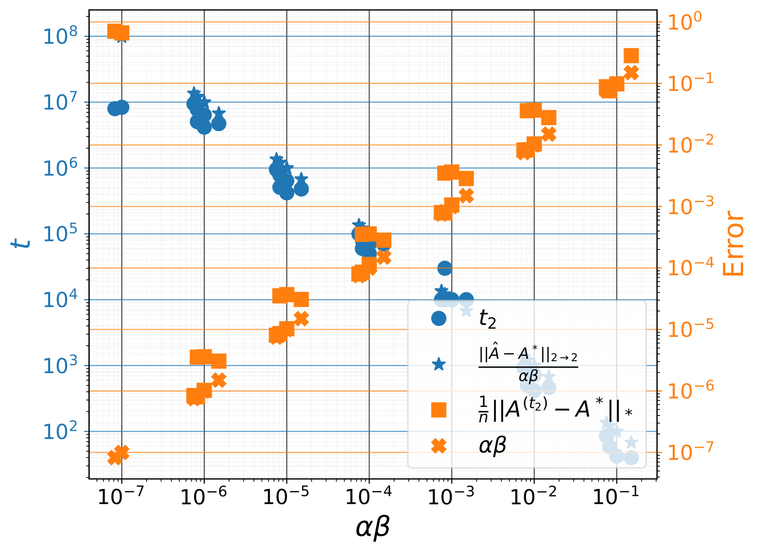
In the noiseless scaling experiment, again let $t_{\mathrm{plat}}$ denote the selected plateau checkpoint. We observe

$$\|\mathbf A^{(t_{\mathrm{plat}})}-\mathbf A^*\|_* \propto\alpha\beta, \qquad t_{\mathrm{plat}} \propto \frac{\|\widehat{\mathbf A}-\mathbf A^*\|_{2\to2}}{\alpha\beta},$$

where $\|\cdot\|_{2\to2}$ is the spectral normThe spectral norm is the largest singular value, equivalently the largest Euclidean stretching factor of the matrix.. If $\mathbf A=\mathbf U\boldsymbol\Sigma\mathbf V^\top$ is a thin singular-value decompositionFor a rank-$r$ matrix, the thin SVD keeps only the $r$ positive singular values and their singular vectors: $\mathbf U\in\mathbb R^{n_1\times r}$, $\boldsymbol\Sigma\in\mathbb R^{r\times r}$, and $\mathbf V\in\mathbb R^{n_2\times r}$., the experiment selects the canonical nuclear-norm subgradient $H(\mathbf A)=\mathbf U\mathbf V^\top$At $\mathbf A=\mathbf U\boldsymbol\Sigma\mathbf V^\top$, the nuclear-norm subdifferential contains $\mathbf U\mathbf V^\top+\mathbf W$ with orthogonality and norm constraints on $\mathbf W$. Choosing $\mathbf W=0$ gives the canonical element.. A pure regularization step decreases each positive singular value by $\alpha\beta$ until discretization causes an $\mathcal O(\alpha\beta)$ oscillation; the small loss gradient perturbs this picture.

We use Wedin’s $\sin\Theta$ perturbation boundWedin’s theorem bounds the angle between singular subspaces of two nearby matrices in terms of the perturbation size divided by an appropriate singular-value gap. (Wedin, 1972) to control the variation of the singular vectors after memorization. When $G(\mathbf A)$ becomes negligible compared with $\beta H(\mathbf A)$, the singular values decay on multiple scales: the smallest singular value converges toward zero first, followed by the next smallest, until $\|\mathbf A^{(t)}\|_*\approx\|\mathbf A^*\|_*$. This process takes $\Theta(1/(\alpha\beta))$ steps. The formal argument is given in the appendix of Notsawo et al. (2025).

Matrix sensing, completion, and data selection

This framework encompasses several matrix-factorization problems. In matrix sensingMatrix sensing observes general linear measurements $\langle\mathbf X_i,\mathbf A^*\rangle$. Matrix completion is the special case in which each measurement reveals one entry of the matrix., one seeks $\mathbf A^*$ from measurement matrices $\{\mathbf X_i\}_{i=1}^N$ and observations

$$y_i^*=\operatorname{tr}(\mathbf X_i^\top\mathbf A^*).$$

In standard matrix completion, each measurement selects one entry: for one-hot row and column vectors $\mathbf x_i^{(1)}$ and $\mathbf x_i^{(2)}$,

$$y_i^*=\mathbf x_i^{(1)\top}\mathbf A^*\mathbf x_i^{(2)}.$$

The recovery guarantees depend on the local coherence and leverage scoresLeverage scores measure how strongly coordinate axes align with the leading row and column singular subspaces. High coherence means that a few entries carry disproportionate information; sampling those entries can be especially valuable in matrix completion. of the compact SVD $\mathbf A^*=\mathbf U^*\boldsymbol\Sigma^*\mathbf V^{*\top}$:

$$\mu_i=\frac{n_1}{r}\|\mathbf U^{*\top}\mathbf e_i\|_2^2, \qquad \nu_j=\frac{n_2}{r}\|\mathbf V^{*\top}\mathbf e_j\|_2^2$$

measure how strongly each row and column aligns with the leading singular subspaces. For $N\leq n_1n_2$ and $\tau\in[0,1]$, we select the first $\tau N$ entries with the largest values of $\mu_i+\nu_j$, then sample the remaining $(1-\tau)N$ entries uniformly from the rest. As $\tau\to1$, performance improves: both the number of examples needed for generalization and the time needed to generalize decrease (Notsawo et al., 2025).

For compressed sensing, the direction is reversed: incoherent measurementsMeasurements that are not aligned with the sparse coordinate basis mix information across coordinates. They reduce redundancy and make different sparse signals easier to distinguish with fewer observations. are beneficial, whereas high coherence between measurement vectors and the sparse basis is detrimental. Thus data selection can amplify or suppress grokking even when the model and optimization hyperparameters remain fixed.

Sparse and low-rank recovery make the point especially clean: generalization is controlled by the property that identifies the hidden object, not by a universal parameter norm.

Grokking without understanding

A late transition can still occur when the active bias is misaligned with the target. Return to sparse recovery, but replace $\ell_1$ regularization with weight decay:

$$f(\mathbf a) = \frac12\|\mathbf X\mathbf a-\mathbf y^*\|_2^2 +\frac\beta2\|\mathbf a\|_2^2.$$

For

$$0<\alpha< \frac{2}{\sigma_{\max}(\mathbf X^\top\mathbf X+\beta\mathbf I_n)},$$

gradient descent converges to the ridge solutionRidge regression adds an $\ell_2^2$ penalty, making the normal-equation matrix invertible when $\beta>0$ and shrinking coefficients toward zero.

$$\widehat{\mathbf a}_\beta = (\mathbf X^\top\mathbf X+\beta\mathbf I_n)^{-1} \mathbf X^\top\mathbf y^*.$$

As $\beta\to0$, this approaches the minimum-Euclidean-norm least-squares solution. If $N<n$, then

$$\|\widehat{\mathbf a}-\mathbf a^*\|_2^2 \geq \|\bigl(\mathbf I_n-\mathbf X^\top(\mathbf X\mathbf X^\top)^\dagger\mathbf X\bigr)\mathbf a^*\|_2^2.$$

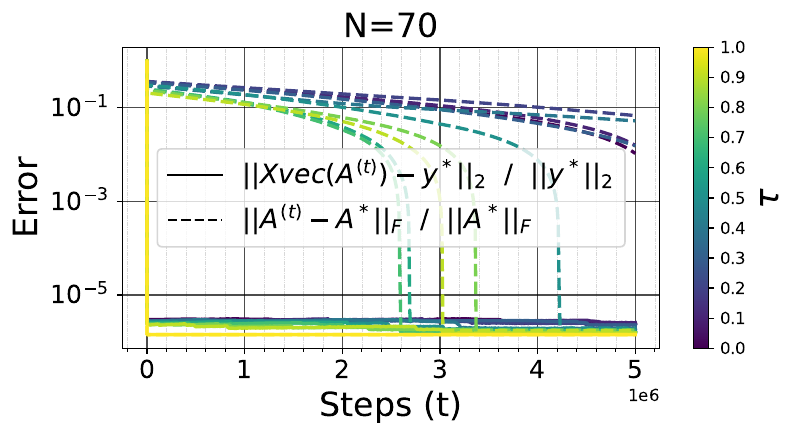
In particular, if $\mathbf a^*$ has a non-zero component orthogonal to the row space of $\mathbf X$The measurements $\mathbf X\mathbf a$ depend only on the projection of $\mathbf a$ onto the row space of $\mathbf X$. Any orthogonal component lies in the null space and is therefore invisible to the data., the minimum-Euclidean-norm solution cannot recover $\mathbf a^*$ perfectly; see Theorem 3.6 of Notsawo et al. (2025). With a large initialization, weight decay can nevertheless produce an abrupt late drop in a proxy error as the parameters move toward $\widehat{\mathbf a}_\beta$.

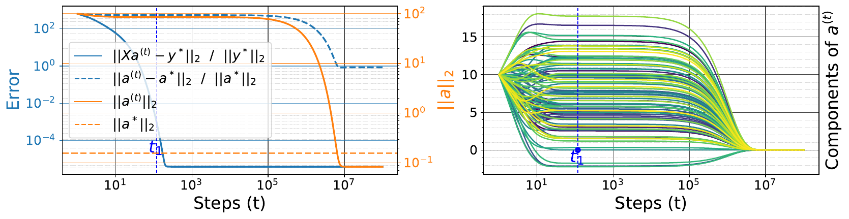
We call this grokking without understanding. A sharp transition in training loss, parameter norm, or another proxy does not establish recovery of the intended rule. The generalization observable must measure what we actually want the model to learn.

The bias need not be an explicit norm

The same mechanism extends beyond an explicit penalty in the objective.

Depth as an implicit bias

In sparse recovery, let $D\geq2$ and parameterize the effective coefficient vector with $\mathbf u_1,\ldots,\mathbf u_D\in\mathbb R^n$ as

$$\mathbf a=\mathbf u_1\odot\cdots\odot\mathbf u_D,$$

where $\odot$ denotes the coordinatewise product. The predictions remain $\mathbf X\mathbf a$, but gradient descent acts on the factors $\mathbf u_1,\ldots,\mathbf u_D$. Depth introduces overparameterization without changing the linear function class. With small initialization, the updates create an implicit preconditioning effectAlthough the predictor is linear in the effective coefficient $\mathbf a$, gradient descent occurs in factor space. Mapping those updates back to $\mathbf a$ produces a state-dependent scaling of coordinates that preferentially amplifies sparse solutions. that promotes sparsity and can recover the target without an explicit $\ell_1$ term. Unlike the shallow case $D=1$, depth can therefore replace $\ell_1$ regularization and permit recovery with fewer measurements.

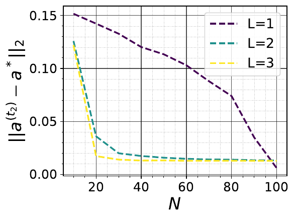
For $D\geq2$, a large initialization combined with small non-zero $\ell_2$ regularization can result in grokking, unlike the shallow case, where we observe grokking without understanding (Notsawo et al., 2025). Related work has established that depth can also produce an implicit low-rank bias in matrix factorization (Gunasekar et al., 2017; Arora et al., 2019; Gidel et al., 2019; Gissin et al., 2019; Razin and Cohen, 2020; Li et al., 2020).

Data selection as an implicit bias

As the matrix-completion experiment above shows, sampling entries with high leverage scores can lower the sample requirement and shorten recovery time. In compressed sensing, choosing measurements incoherent with the sparsifying basis plays the same role. The data determine whether the desired low-complexity solution is identifiable and how quickly it can be reached.

Nonlinear models

The same mechanism appears beyond linear inverse problems.

Algorithmic data

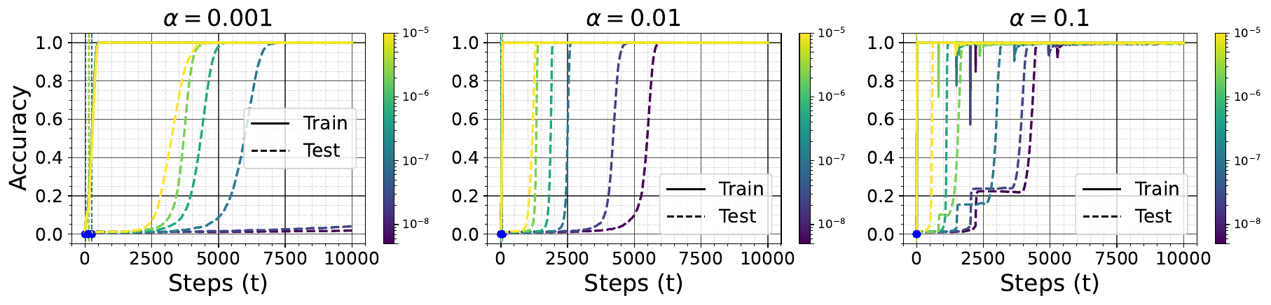
We consider addition modulo $p=97$ with a $40\%$ training fraction, as described in What Is Grokking?. For the MLP, $\ell_1$ and nuclear-norm regularization have the same qualitative effect on grokking as $\ell_2$ regularization: larger values of $\alpha\beta$ lead to faster grokking. The earlier norm-comparison figure varies $\beta$ across all three regularizers; the following figure also varies the learning rate for $\ell_1$ regularization.

Nonlinear teacher–student model

Consider a ReLU teacher

$$\mathbf y^*(\mathbf x)=\mathbf B^*\phi(\mathbf A^*\mathbf x)$$

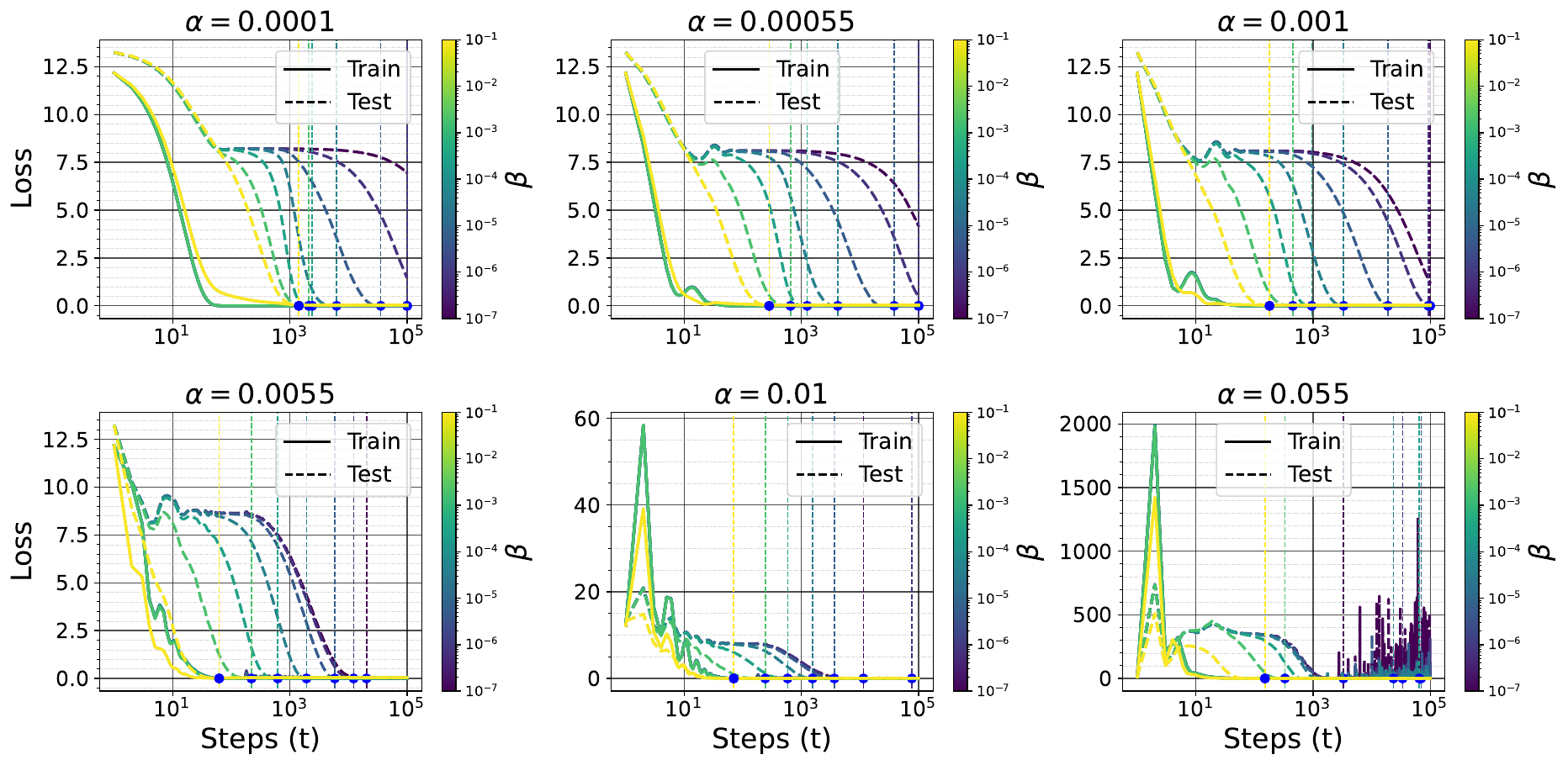
from $\mathbb R^d$ to $\mathbb R^c$ with $r$ hidden neurons, where $\mathbf A^*\in\mathbb R^{r\times d}$, $\mathbf B^*\in\mathbb R^{c\times r}$, and $\phi(z)=\max(z,0)$. We draw $N$ input-output pairs independently and optimize a student $\mathbf y_\theta(\mathbf x)=\mathbf B\phi(\mathbf A\mathbf x)$ from a random normal initialization using

$$g(\theta) = \frac{1}{2N}\sum_{i=1}^N \|\mathbf y_\theta(\mathbf x_i)-\mathbf y^*(\mathbf x_i)\|_2^2.$$

For $\ell_1$, $\ell_2$, and nuclear-norm regularization, the smaller $\alpha\beta$ is, the longer the delay between memorization and generalization. The following representative experiment uses $(d,r,c,N)=(100,500,2,10^2)$ and $\ell_1$ regularization.

Domain-specific regularization

Physics-informed neural networksPINNs use automatic differentiation to evaluate differential-equation residuals and add those residuals to the training objective, encouraging predictions that satisfy the governing equations. incorporate residuals of differential equations into the loss so that solutions remain consistent with physical laws (Raissi et al., 2019). Sobolev trainingSobolev training matches derivatives of the target as well as function values. It therefore controls local behavior that ordinary pointwise supervision may leave unconstrained. extends this idea by matching derivatives of the target function (Czarnecki et al., 2017).

For a student $\mathbf F_\theta$ learning from a teacher $\mathbf F_*$ on inputs $\mathbf x_1,\ldots,\mathbf x_N$, a first-order Sobolev penalty is

$$h(\theta) = \frac1N\sum_{i=1}^N \|\nabla_{\mathbf x}\mathbf F_\theta(\mathbf x_i) -\nabla_{\mathbf x}\mathbf F_*(\mathbf x_i)\|_F^2$$

It favors agreement of input derivatives; $\nabla_{\mathbf x}\mathbf F$ denotes the input JacobianFor a vector-valued function, the input Jacobian is the matrix whose $(i,j)$ entry is $\partial F_i/\partial x_j$. It describes the local sensitivity of every output to every input coordinate.. Here the relevant property is Jacobian agreement, rather than the size of the parameter vector.

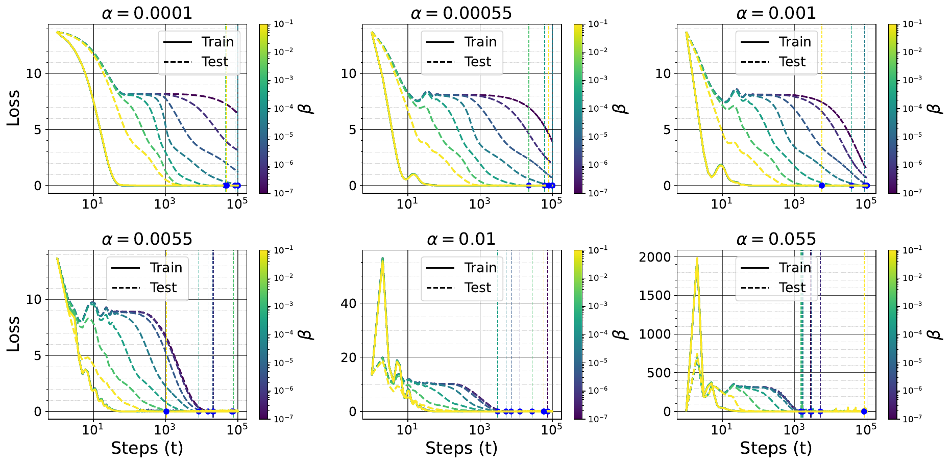
The common structure is simple: the fast dynamics fit the observations; the slow bias selects one fitting solution. Grokking occurs when that selection process eventually favors a solution that generalizes.

References

• Pascal Jr Tikeng Notsawo, Guillaume Dumas, and Guillaume Rabusseau, “Grokking Beyond the Euclidean Norm of Model Parameters”, ICML 2025.
• Stanislav Fort and Adam Scherlis, “The Goldilocks Zone: Towards Better Understanding of Neural Network Loss Landscapes”, 2018.
• Ziming Liu, Eric J. Michaud, and Max Tegmark, “Omnigrok: Grokking Beyond Algorithmic Data”, ICLR 2023.
• Andrey Gromov, “Grokking Modular Arithmetic”, 2023.
• Kaifeng Lyu, Jikai Jin, Zhiyuan Li, Simon S. Du, Jason D. Lee, and Wei Hu, “Dichotomy of Early and Late Phase Implicit Biases Can Provably Induce Grokking”, 2023.
• Tanishq Kumar, Blake Bordelon, Samuel J. Gershman, and Cengiz Pehlevan, “Grokking as the Transition from Lazy to Rich Training Dynamics”, 2023.
• Kaifeng Lyu and Jian Li, “Gradient Descent Maximizes the Margin of Homogeneous Neural Networks”, ICLR 2020.
• Bohan Wang, Qi Meng, Wei Chen, and Tie-Yan Liu, “The Implicit Bias for Adaptive Optimization Algorithms on Homogeneous Neural Networks”, ICML 2021.
• Daniel Kunin, Atsushi Yamamura, Chao Ma, and Surya Ganguli, “The Asymmetric Maximum Margin Bias of Quasi-Homogeneous Neural Networks”, ICLR 2023.
• Sourav Chatterjee, “Convergence of Gradient Descent for Deep Neural Networks”, 2022.
• Chaoyue Liu, Libin Zhu, and Mikhail Belkin, “Loss Landscapes and Optimization in Over-Parameterized Non-Linear Systems and Neural Networks”, 2021.
• Hamed Karimi, Julie Nutini, and Mark Schmidt, “Linear Convergence of Gradient and Proximal-Gradient Methods Under the Polyak–Łojasiewicz Condition”, 2020.
• B. K. Natarajan, “Sparse Approximate Solutions to Linear Systems”, SIAM Journal on Computing 24(2):227–234, 1995.
• David L. Donoho, “Compressed Sensing”, IEEE Transactions on Information Theory 52(4):1289–1306, 2006.
• Venkat Chandrasekaran, Benjamin Recht, Pablo A. Parrilo, and Alan S. Willsky, “The Convex Geometry of Linear Inverse Problems”, Foundations of Computational Mathematics 12(6):805–849, 2012.
• Simon Foucart and Holger Rauhut, A Mathematical Introduction to Compressive Sensing, Birkhäuser Basel, 2013.
• Per-Åke Wedin, “Perturbation Bounds in Connection with Singular Value Decomposition”, BIT Numerical Mathematics 12(1):99–111, 1972.
• Suriya Gunasekar, Blake E. Woodworth, Srinadh Bhojanapalli, Behnam Neyshabur, and Nati Srebro, “Implicit Regularization in Matrix Factorization,” Advances in Neural Information Processing Systems 30, 2017.
• Sanjeev Arora, Nadav Cohen, Wei Hu, and Yuping Luo, “Implicit Regularization in Deep Matrix Factorization”, 2019.
• Gauthier Gidel, Francis Bach, and Simon Lacoste-Julien, “Implicit Regularization of Discrete Gradient Dynamics in Deep Linear Neural Networks”, 2019.
• Daniel Gissin, Shai Shalev-Shwartz, and Amit Daniely, “The Implicit Bias of Depth: How Incremental Learning Drives Generalization”, 2019.
• Noam Razin and Nadav Cohen, “Implicit Regularization in Deep Learning May Not Be Explainable by Norms”, 2020.
• Zhiyuan Li, Yuping Luo, and Kaifeng Lyu, “Towards Resolving the Implicit Bias of Gradient Descent for Matrix Factorization: Greedy Low-Rank Learning”, 2020.
• M. Raissi, P. Perdikaris, and G. E. Karniadakis, “Physics-Informed Neural Networks: A Deep Learning Framework for Solving Forward and Inverse Problems Involving Nonlinear Partial Differential Equations”, Journal of Computational Physics 378:686–707, 2019.
• Wojciech Marian Czarnecki, Simon Osindero, Max Jaderberg, Grzegorz Świrszcz, and Razvan Pascanu, “Sobolev Training for Neural Networks”, 2017.

Cite this post

If you would like to cite this post, you can use the following BibTeX entry:

@misc{tikengnotsawo2025grokkingbeyondl2,
  author = {Tikeng Notsawo, Pascal Jr.},
  title = {{Grokking Beyond the Euclidean Norm of Model Parameters}},
  year = {2025},
  month = jul,
  url = {https://tikquuss.github.io/blog/grokking-beyond-l2/},
  note = {Blog post}
}