Smoothness, Descent, and Cocoercivity

This document provides a rigorous and detailed exploration of smoothness for real-valued functions on $\mathbb{R}^n$, including formal definitions, key lemmas, and proofs. It connects smoothness to Lipschitz continuity of the gradient, descent guarantees in optimization, Hessian bounds, and cocoercivity. The relationships between convexity, smoothness, and cocoercivity are clarified through the Baillon–Haddad theorem.

The central geometric object throughout the article is the affine approximation of $\varphi$ at $\mathbf{x}$,

$$\mathbf{y}\longmapsto \varphi(\mathbf{x})+(\mathbf{y}-\mathbf{x})^\top\nabla\varphi(\mathbf{x}).$$

Convexity specifies on which side of this tangent model the graph lies, while smoothness controls how far from it the graph may move. The quadratic inequalities introduced below make this relationship precise.

Notation

• For a vector $\mathbf{x} \in \mathbb{R}^n$, $\|\mathbf{x}\|_p = \left( \sum_{i=1}^n |\mathbf{x}_i|^{p} \right)^{\frac{1}{p}} \ \forall p \in (0, \infty)$ and $\|\mathbf{x}\|_\infty = \max_{i \in [n]} |\mathbf{x}_i|$.

• For a matrix $\mathbf{A} \in \mathbb{R}^{m \times n}$, we let $\sigma(\mathbf{A}) \subset [0, \infty)$ be the set of singular values of $\mathbf{A}$, and $\sigma_f(\mathbf{A}) = f\{\sigma(\mathbf{A})\}$ for any operator $f \in \{\min,\max,\ldots\}$. Similarly, for a square matrix $\mathbf{A}$, we define $\lambda(\mathbf{A}) \subset \mathbb{R}$ to be its set of eigenvalues.

• For a matrix $\mathbf{A} \in \mathbb{R}^{m \times n}$, the induced $p \rightarrow q$ norm of $\mathbf{A}$ is $\|\mathbf{A}\|_{p \rightarrow q} = \sup_{\mathbf{x} \ne 0 } \frac{\|\mathbf{A}\mathbf{x}\|_q}{\|\mathbf{x}\|_p} = \sup_{\|\mathbf{x}\|_p = 1} \|\mathbf{A}\mathbf{x}\|_q$. We have $\|\mathbf{A}\|_{2 \rightarrow 2} = \sigma_{\max}(\mathbf{A})$, the operator norm, spectral norm, or induced $2$-normThese are three names for the same quantity here: the largest factor by which $\mathbf A$ can stretch a Euclidean unit vector. It equals the largest singular value $\sigma_{\max}(\mathbf A)$..

Definition 1 [Subdifferentiability]

A function $\varphi : \mathbb{R}^n \to \mathbb{R}$ is said to be subdifferentiable at $\mathbf{x} \in \mathbb{R}^n$ if and only if

$$\exists \mathbf{z} \in \mathbb{R}^n, \quad \varphi(\mathbf{y}) \ge \varphi(\mathbf{x}) + (\mathbf{y} - \mathbf{x})^\top \mathbf{z} \quad \forall \mathbf{y} \in \mathbb{R}^n$$

The set of all such $\mathbf{z}$ is called the subdifferential of $\varphi$ at $\mathbf{x}$ and is denoted by $\partial \varphi(\mathbf{x})$. When $\partial \varphi(\mathbf{x})$ is a singleton, we say that $\varphi$ is differentiable at $\mathbf{x}$:

$$\partial \varphi(\mathbf{x}) = \{ \nabla \varphi(\mathbf{x})\}$$ $$\begin{array}{r} \blacksquare\Box \end{array}$$

The vector $\mathbf{z}$ specifies the slope of the affine function

$$\mathbf{y}\longmapsto \varphi(\mathbf{x})+(\mathbf{y}-\mathbf{x})^\top\mathbf{z}.$$

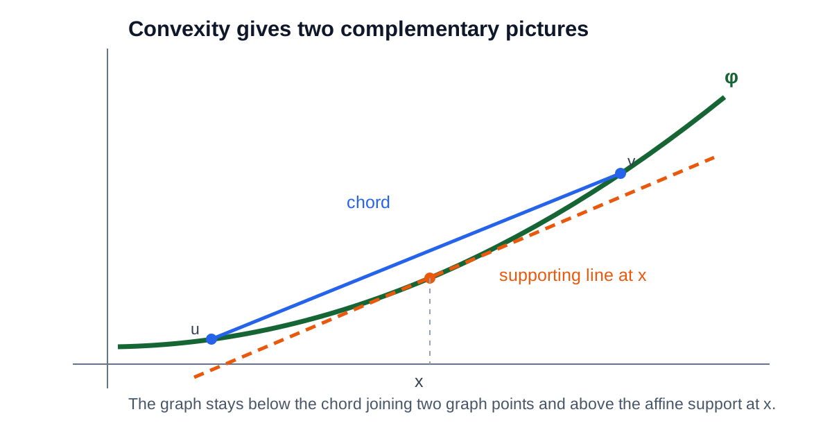
The defining inequality says that this affine function supports the graph of $\varphi$ from below: it touches the graph at $\mathbf{x}$ and never crosses above it. In one dimension, it is a supporting line; in higher dimensions, it is a supporting hyperplane. The subdifferential collects every slope that can provide such a support.

Definition 2 [Convexity]

A function $\varphi : \mathbb{R}^n \to \mathbb{R}$ is said to be convex if and only if

$$\varphi\left(\lambda \mathbf{x} + (1 - \lambda)\mathbf{y} \right) \le \lambda \varphi(\mathbf{x}) + (1 - \lambda)\varphi(\mathbf{y}) \quad \forall \mathbf{x}, \mathbf{y} \in \mathbb{R}^n, \quad \forall \lambda \in (0,1)$$

If $\varphi$ is subdifferentiable, convexity implies

$$\varphi(\mathbf{y}) \ge \varphi(\mathbf{x}) + (\mathbf{y}-\mathbf{x})^\top \mathbf{z} \quad \forall \mathbf{x}, \mathbf{y} \in \mathbb{R}^n, \quad \forall \mathbf{z} \in \partial \varphi(\mathbf{x})$$

If $\varphi$ is twice differentiable, convexity implies

$$\lambda_{\min}\left( \nabla^2 \varphi(\mathbf{x}) \right) \ge 0 \quad \forall \mathbf{x} \in \mathbb{R}^n$$ $$\begin{array}{r} \blacksquare\Box \end{array}$$

The defining inequality says that the graph of a convex function lies below every chord joining two points of its graph. When the function is differentiable, the equivalent first-order picture is that every tangent hyperplane lies below the graph. When it is twice differentiable, the nonnegative eigenvalues of the Hessian say that the function bends upward in every direction.

Definition 3 [Lipschitz Continuity]

For $L > 0$, a function $\Phi : \mathbb{R}^n \to \mathbb{R}^m$ is $L$-Lipschitz continuous if and only if

$$\begin{equation} \|\Phi (\mathbf{y}) - \Phi (\mathbf{x}) \|_2 \le L \|\mathbf{y}-\mathbf{x}\|_2 \quad \forall \mathbf{x}, \mathbf{y} \in \mathbb{R}^n \end{equation}$$

When $L=1$, this means that $\Phi$ is nonexpansiveA nonexpansive map never increases pairwise distance: $\|\Phi(\mathbf y)-\Phi(\mathbf x)\|_2\le\|\mathbf y-\mathbf x\|_2$..

$$\begin{array}{r} \blacksquare\Box \end{array}$$

The inequality compares two distances: the distance between the inputs and the distance between their images. The map may rotate, bend, or collapse space, but it cannot separate two outputs by more than $L$ times the original input separation. Thus, $L$ is a worst-case amplification factor. When $L=1$, no pairwise distance can increase, which explains the term nonexpansive.

When $\Phi=\nabla\varphi$, Lipschitz continuity means that the slope of $\varphi$ cannot change arbitrarily fast as the point moves.

Definition 4 [Cocoercivity]

For $L > 0$, a vector field $\Phi : \mathbb{R}^n \to \mathbb{R}^n$ is $1/L$-cocoercive if and only if

$$\langle \Phi(\mathbf{x})-\Phi(\mathbf{y}),\mathbf{x}-\mathbf{y}\rangle \ge \frac{1}{L}\|\Phi(\mathbf{x})-\Phi(\mathbf{y})\|_2^2 \quad \forall \mathbf{x},\mathbf{y}\in\mathbb{R}^n$$

Cocoercivity is also often called the Dunn property or inverse strong monotonicityThe names emphasize two equivalent viewpoints: cocoercivity is historically associated with Dunn, and it can be read as strong monotonicity of the inverse relation when that inverse is well defined.. When $L=1$, this means that $\Phi$ is firmly nonexpansiveA map is firmly nonexpansive when $\|\Phi(\mathbf x)-\Phi(\mathbf y)\|_2^2\le\langle\Phi(\mathbf x)-\Phi(\mathbf y),\mathbf x-\mathbf y\rangle$. This is stronger than ordinary nonexpansiveness..

$$\begin{array}{r} \blacksquare\Box \end{array}$$

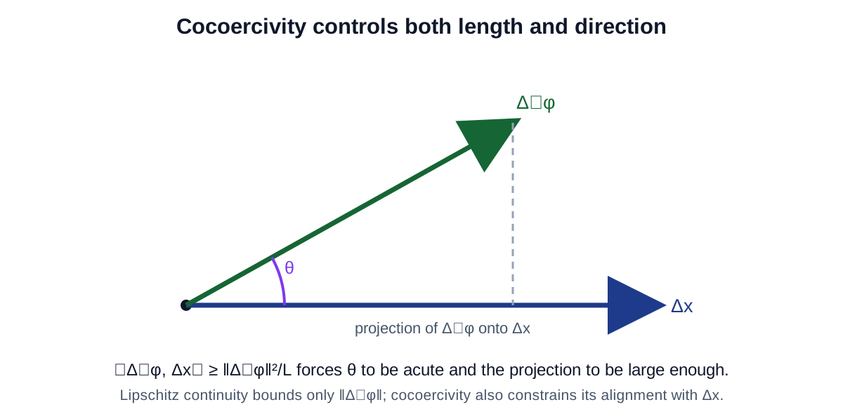
Write $\boldsymbol{\Delta}_x:=\mathbf{x}-\mathbf{y}$ and $\boldsymbol{\Delta}_\Phi:=\Phi(\mathbf{x})-\Phi(\mathbf{y})$. Lipschitz continuity controls only the length of $\boldsymbol{\Delta}_\Phi$. Cocoercivity also controls its direction: the inner product requires $\boldsymbol{\Delta}_\Phi$ to have a sufficiently large component along $\boldsymbol{\Delta}_x$. In particular, the inner product is nonnegative, so a cocoercive field is monotone.

By the Cauchy–Schwarz inequality, cocoercivity implies $\|\boldsymbol{\Delta}_\Phi\|_2 \le L\|\boldsymbol{\Delta}_x\|_2$. Thus, cocoercivity is stronger than $L$-Lipschitz continuity in general. The Baillon–Haddad theorem will show that the two notions become equivalent for gradients of convex functions.

Definition 5 [Smoothness]

For $L > 0$, a differentiable function $\varphi : \mathbb{R}^n \to \mathbb{R}$ is $L$-smooth if and only if $\nabla \varphi : \mathbb{R}^n \to \mathbb{R}^n$ is $L$-Lipschitz continuous.

$$\begin{array}{r} \blacksquare\Box \end{array}$$

The word smooth refers here to the controlled variation of the gradient, not to the mere existence of many derivatives. If one moves a distance $r$, the gradient can change by at most $Lr$. Consequently, the function cannot bend upward or downward faster than a quadratic with curvature $L$. This is why $L$ appears in the quadratic envelopes of Definition 6 and in the step-size threshold $2/L$ of the descent and ascent lemma below. A small $L$ means that the tangent model remains accurate over a relatively large neighborhood. A large $L$ permits the slope to change rapidly, so a smaller optimization step is needed.

Remark 1

In classical analysis and differential geometry, a function $\varphi : \mathbb{R}^n \to \mathbb{R}$ is often called smooth if it belongs to $C^\infty(\mathbb{R}^n)$$C^\infty$ is a local differentiability condition of every order. $L$-smoothness is a global quantitative bound on how fast the first derivative changes. Neither property implies the other on all of $\mathbb R^n$., meaning that all its partial derivatives of every order exist and are continuous. This notion differs from $L$-smoothness in optimization, which only requires the gradient to be $L$-Lipschitz continuous. Neither property implies the other in general:

• A $C^\infty$ function need not have a globally Lipschitz gradient. For example, $\varphi(\mathbf{x})=x_1^4$ belongs to $C^\infty(\mathbb{R}^n)$, but its Hessian $\nabla^2\varphi(\mathbf{x})=12x_1^2\mathbf{e}_1\mathbf{e}_1^\top$ is unbounded. Hence, $\nabla\varphi$ is not globally Lipschitz.

• An $L$-smooth function need not belong to $C^\infty$. For example, $\varphi(\mathbf{x})=x_1^2\mathbb{1}_{\{x_1>0\}}$ is $2$-smooth, but it is not twice differentiable at points where $x_1=0$, and therefore does not belong to $C^2(\mathbb{R}^n)\supsetneq C^\infty(\mathbb{R}^n)$.

Definition 6 [$L$-UQI, $L$-LQI, and $L$-QI]

For $L>0$, a differentiable function $\varphi:\mathbb{R}^n\to\mathbb{R}$

• is $L$-UQI (upper quadratic inequality) if and only if

$$\begin{equation} \varphi(\mathbf{y})-\Big[\varphi(\mathbf{x})+(\mathbf{y}-\mathbf{x})^\top\nabla\varphi(\mathbf{x})\Big] \le \frac{L}{2}\|\mathbf{y}-\mathbf{x}\|_2^2 \quad \forall \mathbf{x},\mathbf{y}\in\mathbb{R}^n \tag{$L$-UQI} \end{equation}$$

• is $L$-LQI (lower quadratic inequality) if and only if

$$\begin{equation} -\frac{L}{2}\|\mathbf{y}-\mathbf{x}\|_2^2 \le \varphi(\mathbf{y})-\Big[\varphi(\mathbf{x})+(\mathbf{y}-\mathbf{x})^\top\nabla\varphi(\mathbf{x})\Big] \quad \forall \mathbf{x},\mathbf{y}\in\mathbb{R}^n \tag{$L$-LQI} \end{equation}$$

• is $L$-QI (quadratic inequality) if and only if it is both $L$-UQI and $L$-LQI, equivalently,

$$\begin{equation} \left|\varphi(\mathbf{y})-\Big[\varphi(\mathbf{x})+(\mathbf{y}-\mathbf{x})^\top\nabla\varphi(\mathbf{x})\Big]\right| \le \frac{L}{2}\|\mathbf{y}-\mathbf{x}\|_2^2 \quad \forall \mathbf{x},\mathbf{y}\in\mathbb{R}^n \tag{$L$-QI} \end{equation}$$ $$\begin{array}{r} \blacksquare\Box \end{array}$$

For a base point $\mathbf{x}$, define the first-order Taylor remainder

$$R_\varphi(\mathbf{y};\mathbf{x}) :=\varphi(\mathbf{y})- \Big[\varphi(\mathbf{x})+(\mathbf{y}-\mathbf{x})^\top\nabla\varphi(\mathbf{x})\Big].$$

This is the vertical error made when the tangent model at $\mathbf{x}$ is used to predict the value at $\mathbf{y}$.

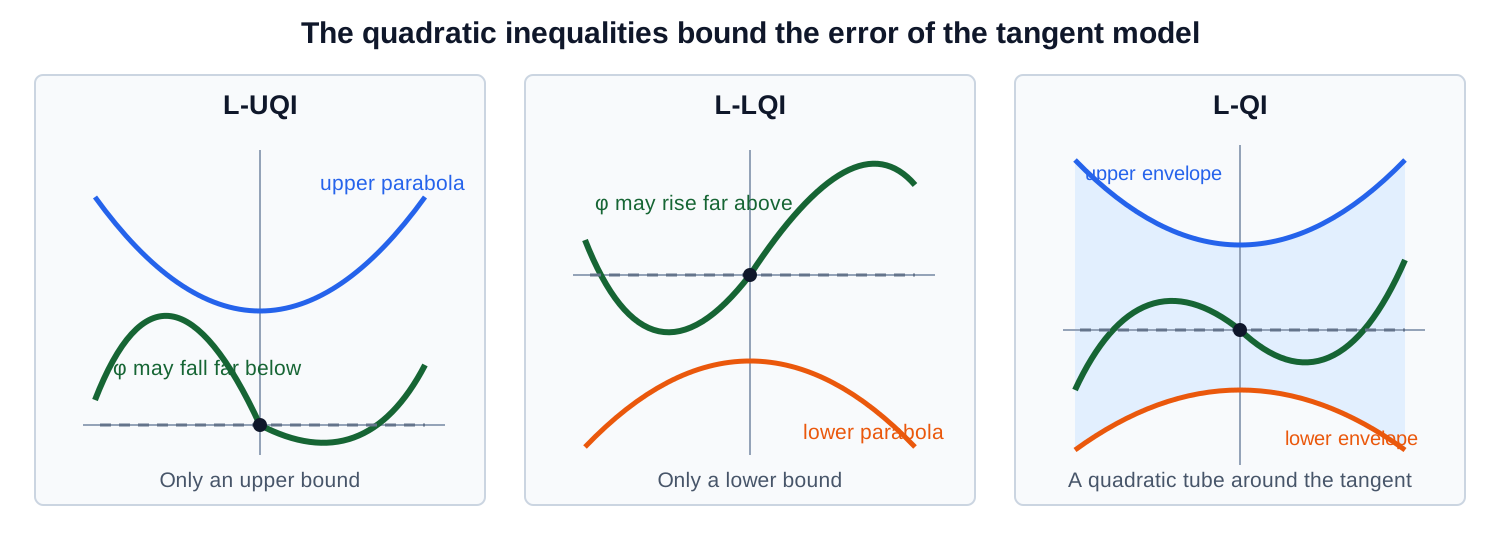
• $L$-UQI literally means that this error is bounded from above by $(L/2)\|\mathbf{y}-\mathbf{x}\|_2^2$. Geometrically, the graph cannot rise above the upward quadratic model centered at $\mathbf{x}$. It may, however, fall arbitrarily far below that model.

• $L$-LQI means that the error is bounded from below by $-(L/2)\|\mathbf{y}-\mathbf{x}\|_2^2$. Geometrically, the graph cannot fall below the downward quadratic model. It may rise arbitrarily far above it.

• $L$-QI imposes both bounds. The graph is trapped inside a quadratic tube around its tangent model, and the approximation error grows at most quadratically with the distance from $\mathbf{x}$.

These inequalities do not, by themselves, assert convexity. Convexity would additionally require $R_\varphi(\mathbf{y};\mathbf{x})\ge0$, whereas concavity would require $R_\varphi(\mathbf{y};\mathbf{x})\le0$.

Definition 7 [$L$-GLB and $L$-GUB]

For $L>0$, a differentiable function $\varphi:\mathbb{R}^n\to\mathbb{R}$

• is $L$-GLB (gradient lower bound) if and only if

$$\begin{equation} \frac{1}{2L}\|\nabla\varphi(\mathbf{y})-\nabla\varphi(\mathbf{x})\|_2^2 \le \varphi(\mathbf{y})-\varphi(\mathbf{x}) -(\mathbf{y}-\mathbf{x})^\top\nabla\varphi(\mathbf{x}) \quad \forall \mathbf{x},\mathbf{y}\in\mathbb{R}^n \tag{$L$-GLB} \end{equation}$$

• is $L$-GUB (gradient upper bound) if and only if

$$\begin{equation} \varphi(\mathbf{y})-\varphi(\mathbf{x}) -(\mathbf{y}-\mathbf{x})^\top\nabla\varphi(\mathbf{x}) \le -\frac{1}{2L}\|\nabla\varphi(\mathbf{y})-\nabla\varphi(\mathbf{x})\|_2^2 \quad \forall \mathbf{x},\mathbf{y}\in\mathbb{R}^n \tag{$L$-GUB} \end{equation}$$ $$\begin{array}{r} \blacksquare\Box \end{array}$$

The $L$-GLB and $L$-GUB relate two changes at once: the error of the tangent model and the change in the gradient. The $L$-GLB says that a positive tangent-model error must be large enough to account for the squared change in slope. Its concave counterpart, the $L$-GUB, says the same thing after reversing the sign.

For a convex $L$-smooth function, the $L$-GLB strengthens the ordinary supporting-hyperplane inequality $0\le R_\varphi(\mathbf{y};\mathbf{x})$ to $\frac{1}{2L}\|\nabla\varphi(\mathbf{y})-\nabla\varphi(\mathbf{x})\|_2^2 \le R_\varphi(\mathbf{y};\mathbf{x})$. Thus, a large change in gradient requires a correspondingly large gap above the tangent hyperplane.

Lemma 1 [One-sided QI]

Let $L>0$ and let $f:\mathbb{R}^n\to\mathbb{R}$ be differentiable.

• Being $L$-UQI alone, or $L$-LQI alone, does not imply $L$-smoothness in general.

• If $f$ is convex and $L$-UQI, then $f$ is $L$-smooth and $L$-GLB.

• If $f$ is concave and $L$-LQI, then $f$ is $L$-smooth and $L$-GUB.

Remark 2

This lemma says that one-sided quadratic inequality controls curvature in only one direction. The $L$-UQI prevents excessive upward bending but allows arbitrarily strong downward bending; the $L$-LQI does the reverse. This is why neither condition alone guarantees $L$-smoothness.

Convexity supplies the missing sign: for a convex differentiable function, $0\le R_f(\mathbf{y};\mathbf{x})$. Combining this with the $L$-UQI traps the remainder between $0$ and $(L/2)\|\mathbf{y}-\mathbf{x}\|_2^2$. For a concave function, the symmetric argument combines the nonpositivity of the remainder with the $L$-LQI. The counterexamples at the end of the proof show exactly what fails when this curvature sign is absent.

Proof

Convex case.

Fix $\mathbf{x},\mathbf{y}\in\mathbb{R}^n$ and define the affine shiftAdding or subtracting an affine function does not change curvature: the affine term cancels in the convexity inequality. Thus $F_{\mathbf x}$ is convex whenever $f$ is convex.

$$F_{\mathbf{x}}(\mathbf{z}) :=f(\mathbf{z})-f(\mathbf{x}) -(\mathbf{z}-\mathbf{x})^\top\nabla f(\mathbf{x}).$$

By convexity, $F_{\mathbf{x}}(\mathbf{z})\ge 0$ for every $\mathbf{z}\in\mathbb{R}^n$. Subtracting an affine function preserves the $L$-UQI, so

$$F_{\mathbf{x}}(\mathbf{v}) \le F_{\mathbf{x}}(\mathbf{u}) +(\mathbf{v}-\mathbf{u})^\top\nabla F_{\mathbf{x}}(\mathbf{u}) +\frac{L}{2}\|\mathbf{v}-\mathbf{u}\|_2^2 \quad \forall \mathbf{u},\mathbf{v}\in\mathbb{R}^n.$$

Set

$$\mathbf{s}:=\nabla F_{\mathbf{x}}(\mathbf{y}) =\nabla f(\mathbf{y})-\nabla f(\mathbf{x}), \qquad \mathbf{w}:=\mathbf{y}-\frac{1}{L}\mathbf{s}.$$

Applying the $L$-UQI for $F_{\mathbf{x}}$ with base point $\mathbf{y}$ and target point $\mathbf{w}$ gives

$$\begin{equation} \begin{aligned} 0\le F_{\mathbf{x}}(\mathbf{w}) &\le F_{\mathbf{x}}(\mathbf{y}) +(\mathbf{w}-\mathbf{y})^\top\mathbf{s} +\frac{L}{2}\|\mathbf{w}-\mathbf{y}\|_2^2 \\ &=F_{\mathbf{x}}(\mathbf{y}) +\textcolor{#2563eb}{\left(-\frac{1}{L}\mathbf{s}\right)^\top\mathbf{s}} +\frac{L}{2}\left\|\textcolor{#2563eb}{-\frac{1}{L}\mathbf{s}}\right\|_2^2 \\ &=F_{\mathbf{x}}(\mathbf{y})-\frac{1}{2L}\|\mathbf{s}\|_2^2. \end{aligned} \end{equation}$$

The blue terms show the substitution $\mathbf{w}-\mathbf{y}=-\mathbf{s}/L$ in both the linear and quadratic terms. Their contributions combine to $-\|\mathbf{s}\|_2^2/(2L)$.

Rearranging and recalling that $\mathbf{s}=\nabla f(\mathbf{y})-\nabla f(\mathbf{x})$ gives

$$\begin{equation} \frac{1}{2L}\|\nabla f(\mathbf{y})-\nabla f(\mathbf{x})\|_2^2 \le F_{\mathbf{x}}(\mathbf{y}) =f(\mathbf{y})-f(\mathbf{x}) -(\mathbf{y}-\mathbf{x})^\top\nabla f(\mathbf{x}), \end{equation}$$

which explicitly proves that $f$ is $L$-GLB. On the other hand, since $f$ is $L$-UQI,

$$\begin{equation} F_{\mathbf{x}}(\mathbf{y})\le\frac{L}{2}\|\mathbf{y}-\mathbf{x}\|_2^2. \end{equation}$$

Combining these two displayed inequalities yields

$$\frac{1}{2L}\|\nabla f(\mathbf{y})-\nabla f(\mathbf{x})\|_2^2 \le\frac{L}{2}\|\mathbf{y}-\mathbf{x}\|_2^2.$$

Because $L>0$, taking square roots gives

$$\|\nabla f(\mathbf{y})-\nabla f(\mathbf{x})\|_2 \le L\|\mathbf{y}-\mathbf{x}\|_2.$$

Thus $f$ is $L$-smooth.

Concave case.

Assume that $f$ is concave and $L$-LQI, and apply the sign reversal $q:=-f$Negation turns concavity into convexity, changes a lower quadratic inequality into an upper one, and preserves gradient differences up to sign. It therefore transfers the convex result directly to the concave case.. Then $q$ is convex, and the $L$-LQI for $f$ is equivalent to the $L$-UQI for $q$. By the convex case, $q$ is $L$-smooth and $L$-GLB. Since $\nabla q=-\nabla f$, it follows immediately that $f$ is $L$-smooth. The $L$-GLB for $q$ gives

$$\frac{1}{2L}\|\nabla f(\mathbf{y})-\nabla f(\mathbf{x})\|_2^2 \le -\left[f(\mathbf{y})-f(\mathbf{x}) -(\mathbf{y}-\mathbf{x})^\top\nabla f(\mathbf{x})\right],$$

which is equivalent to the $L$-GUB for $f$.

Counterexamples: why a one-sided quadratic inequality is insufficient

For the $L$-UQI, let $f:\mathbb{R}^n\to\mathbb{R}$ be defined by

$$f(\mathbf{x}):=-a\|\mathbf{x}\|_2^2 \qquad (a>0).$$

Then $\nabla f(\mathbf{x})=-2a\mathbf{x}$ and, for every $\mathbf{x},\mathbf{y}\in\mathbb{R}^n$,

$$\begin{equation} f(\mathbf{y})-f(\mathbf{x}) -(\mathbf{y}-\mathbf{x})^\top\nabla f(\mathbf{x}) =-a\|\mathbf{y}-\mathbf{x}\|_2^2 \le \frac{L}{2}\|\mathbf{y}-\mathbf{x}\|_2^2. \end{equation}$$

Thus $f$ is $L$-UQI for every $L>0$. However,

$$\|\nabla f(\mathbf{y})-\nabla f(\mathbf{x})\|_2 =2a\|\mathbf{y}-\mathbf{x}\|_2,$$

so $f$ is $L$-smooth if and only if $L\ge 2a$. Choosing $0<L<2a$ shows that the $L$-UQI alone does not imply $L$-smoothness.

For the $L$-LQI, define instead $f(\mathbf{x}):=a\|\mathbf{x}\|_2^2$. Then

$$\begin{equation} f(\mathbf{y})-f(\mathbf{x}) -(\mathbf{y}-\mathbf{x})^\top\nabla f(\mathbf{x}) =a\|\mathbf{y}-\mathbf{x}\|_2^2 \ge -\frac{L}{2}\|\mathbf{y}-\mathbf{x}\|_2^2. \end{equation}$$

so $f$ is $L$-LQI. Again, $f$ is $L$-smooth if and only if $L\ge 2a$. Choosing $0<L<2a$ shows that the $L$-LQI alone does not imply $L$-smoothness.

$$\begin{array}{r} \blacksquare\Box \end{array}$$

Lemma 2 [Descent and Ascent Lemma]

Let $L>0$, and let $\varphi:\mathbb{R}^n\to\mathbb{R}$ be differentiable. Then $\varphi$ is $L$-smooth if and only if it is $L$-QI.

Remark 3

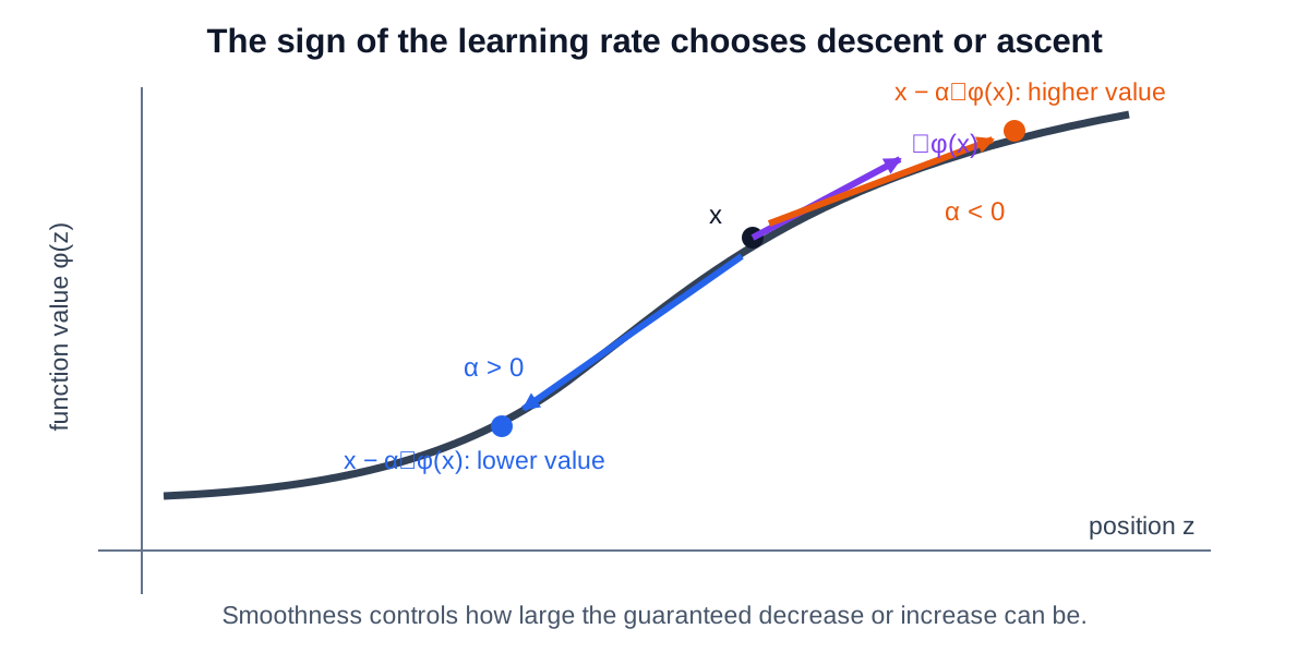
The standard descent lemma in the optimization literature usually focuses on only one side of the result: the upper quadratic inequality and the descent obtained with a positive learning rate. Here, we state the two-sided $L$-QI and thus generalize the usual presentation to include ascent as well. Indeed, for any learning rate $\alpha\in[0,2/L]$, moving from $\mathbf{x}$ to $\mathbf{x}-\alpha\nabla\varphi(\mathbf{x})$ cannot increase $\varphi$. Symmetrically, for $\alpha\in[-2/L,0]$, the same update moves in the gradient direction and cannot decrease $\varphi$. Corollary 1 quantifies both the descent and the ascent, while Corollary 2 gives the corresponding gradient bounds when $\varphi$ is bounded below or bounded above.

The equivalence is important: $L$-smoothness is a statement about the variation of the gradient, whereas the $L$-QI is a statement about function values and tangent models. Lemma 2 says that these are two descriptions of exactly the same regularity.

Proof

($\Longrightarrow$) $L$-smoothness implies $L$-QI.

Let $\mathbf{x}, \mathbf{y} \in \mathbb{R}^n$ and define $\mathbf{d}:=\mathbf{y}-\mathbf{x}$. We reduce the multivariate statement to the one–variable case by slicing $\varphi$ along the line segment joining $\mathbf{x}$ and $\mathbf{y}$. Define $\psi:[0,1] \longrightarrow \mathbb{R}$ by

$$\psi(t) = \varphi\left(\mathbf{x}+t\mathbf{d}\right).$$

By the fundamental theorem of calculus, $\psi(1)=\psi(0)+\int_0^1\psi'(t)dt$, and by the chain rule, $\psi'(t)=\left\langle\nabla\varphi\left(\mathbf{x}+t\mathbf{d}\right),\mathbf{d}\right\rangle$. Therefore,

$$\begin{equation} \begin{aligned} \varphi(\mathbf{y}) &=\varphi(\mathbf{x}) +\int_0^1\left\langle\nabla\varphi(\mathbf{x}+t\mathbf{d}),\mathbf{d}\right\rangle dt \\ &=\varphi(\mathbf{x}) +\textcolor{#2563eb}{\left\langle\nabla\varphi(\mathbf{x}),\mathbf{d}\right\rangle} +\int_0^1\left\langle \nabla\varphi(\mathbf{x}+t\mathbf{d}) \textcolor{#2563eb}{-\nabla\varphi(\mathbf{x})},\mathbf{d}\right\rangle dt \\ &\le \varphi(\mathbf{x}) +\left\langle\nabla\varphi(\mathbf{x}),\mathbf{d}\right\rangle +\int_0^1 \left\|\nabla\varphi(\mathbf{x}+t\mathbf{d})-\nabla\varphi(\mathbf{x})\right\|_2 \|\mathbf{d}\|_2 dt \\ &\le \varphi(\mathbf{x}) +\left\langle\nabla\varphi(\mathbf{x}),\mathbf{d}\right\rangle +\int_0^1 L\|\mathbf{x}+t\mathbf{d}-\mathbf{x}\|_2\|\mathbf{d}\|_2 dt \\ &=\varphi(\mathbf{x}) +\left\langle\nabla\varphi(\mathbf{x}),\mathbf{d}\right\rangle +L\|\mathbf{d}\|_2^2\int_0^1t\,dt \\ &=\varphi(\mathbf{x}) +\left\langle\nabla\varphi(\mathbf{x}),\mathbf{d}\right\rangle +\frac{L}{2}\|\mathbf{d}\|_2^2. \end{aligned} \end{equation}$$

In the second equality, the blue terms display the same quantity being added and subtracted. The first inequality follows from the Cauchy–Schwarz inequality, and the second uses the $L$-Lipschitz continuity of $\nabla\varphi$.

Since $-\varphi$ is also $L$-smooth, applying the upper bound just proved to $-\varphi$ gives

$$\begin{equation} -\varphi(\mathbf{y}) \le -\varphi(\mathbf{x}) -\left\langle\nabla\varphi(\mathbf{x}),\mathbf{d}\right\rangle +\frac{L}{2}\|\mathbf{d}\|_2^2, \end{equation}$$

or, equivalently,

$$\begin{equation} \varphi(\mathbf{y}) \ge \varphi(\mathbf{x}) +\left\langle\nabla\varphi(\mathbf{x}),\mathbf{d}\right\rangle -\frac{L}{2}\|\mathbf{d}\|_2^2. \end{equation}$$

Combining the upper and lower bounds and recalling that $\mathbf{d}=\mathbf{y}-\mathbf{x}$ yields precisely the two-sided $L$-QI.

($\Longleftarrow$) $L$-QI implies $L$-smoothness.

Assume that $\varphi$ is $L$-QI. Fix $\mathbf{x},\mathbf{y}\in\mathbb{R}^n$ and set

$$\mathbf{d}:=\mathbf{y}-\mathbf{x}, \qquad r:=\varphi(\mathbf{y})-\varphi(\mathbf{x}) -\left\langle\nabla\varphi(\mathbf{x}),\mathbf{d}\right\rangle.$$

The $L$-QI gives $|r|\le (L/2)\|\mathbf{d}\|_2^2$. Define

$$g(\mathbf{z}):=\varphi(\mathbf{z})+\frac{L}{2}\|\mathbf{z}\|_2^2, \qquad h(\mathbf{z}):=-\varphi(\mathbf{z})+\frac{L}{2}\|\mathbf{z}\|_2^2.$$

Their first-order remainders are

$$\begin{equation} \begin{aligned} g(\mathbf{y})-g(\mathbf{x}) -\left\langle\nabla g(\mathbf{x}),\mathbf{d}\right\rangle &=\textcolor{#2563eb}{r}+\textcolor{#7c3aed}{\frac{L}{2}\|\mathbf{d}\|_2^2}, \\ h(\mathbf{y})-h(\mathbf{x}) -\left\langle\nabla h(\mathbf{x}),\mathbf{d}\right\rangle &=\textcolor{#ea580c}{-r}+\textcolor{#7c3aed}{\frac{L}{2}\|\mathbf{d}\|_2^2}. \end{aligned} \end{equation}$$

The blue and orange terms are the two possible signs of the same remainder $r$, while the purple quadratic term is common to both shifted functions. Since $|r|\le(L/2)\|\mathbf{d}\|_2^2$, both colored sums are nonnegative.

Both quantities lie in $[0,L\|\mathbf{d}\|_2^2]$. Hence $g$ and $h$ are convex and $2L$-UQI. By Lemma 1, they are $(2L)$-GLB. Therefore,

$$\begin{equation} \begin{aligned} \frac{1}{4L}\|\nabla g(\mathbf{y})-\nabla g(\mathbf{x})\|_2^2 &\le g(\mathbf{y})-g(\mathbf{x}) -\left\langle\nabla g(\mathbf{x}),\mathbf{d}\right\rangle, \\ \frac{1}{4L}\|\nabla h(\mathbf{y})-\nabla h(\mathbf{x})\|_2^2 &\le h(\mathbf{y})-h(\mathbf{x}) -\left\langle\nabla h(\mathbf{x}),\mathbf{d}\right\rangle. \end{aligned} \end{equation}$$

Let $\boldsymbol{\Delta}:=\nabla\varphi(\mathbf{y})-\nabla\varphi(\mathbf{x})$. Then

$$\nabla g(\mathbf{y})-\nabla g(\mathbf{x}) =\textcolor{#2563eb}{\boldsymbol{\Delta}+L\mathbf{d}}, \qquad \nabla h(\mathbf{y})-\nabla h(\mathbf{x}) =\textcolor{#ea580c}{-\boldsymbol{\Delta}+L\mathbf{d}}.$$

Adding the two preceding inequalities and using the parallelogram identityFor vectors $\mathbf a$ and $\mathbf b$, $\|\mathbf a+\mathbf b\|_2^2+\|\mathbf a-\mathbf b\|_2^2=2\|\mathbf a\|_2^2+2\|\mathbf b\|_2^2$. The opposite cross terms cancel. gives

$$\begin{equation} \begin{aligned} \frac{1}{4L} \left(\textcolor{#2563eb}{\|\boldsymbol{\Delta}+L\mathbf{d}\|_2^2} +\textcolor{#ea580c}{\|-\boldsymbol{\Delta}+L\mathbf{d}\|_2^2}\right) &\le L\|\mathbf{d}\|_2^2 \\ \Longleftrightarrow\quad \|\boldsymbol{\Delta}\|_2^2+L^2\|\mathbf{d}\|_2^2 &\le 2L^2\|\mathbf{d}\|_2^2 \\ \Longrightarrow\quad \|\boldsymbol{\Delta}\|_2 &\le L\|\mathbf{d}\|_2. \end{aligned} \end{equation}$$

The blue and orange vectors are mirror images in the $\boldsymbol{\Delta}$ component. When their squared norms are added, the opposite cross terms cancel; this is precisely the parallelogram identity used in the next line.

Thus $\nabla\varphi$ is $L$-Lipschitz continuous, so $\varphi$ is $L$-smooth.

$$\begin{array}{r} \blacksquare\Box \end{array}$$

Corollary 1 [Descent and ascent]

If a function $\varphi:\mathbb{R}^n\to\mathbb{R}$ is $L$-smooth, then, for every $\mathbf{x}\in\mathbb{R}^n$ and every $\alpha\in\mathbb{R}$,

$$\begin{equation} \begin{aligned} \varphi(\mathbf{x})- \frac{\alpha(2+L\alpha)}{2}\|\nabla\varphi(\mathbf{x})\|_2^2 &\le \varphi\bigl(\mathbf{x}-\alpha\nabla\varphi(\mathbf{x})\bigr) \\ &\le \varphi(\mathbf{x})- \frac{\alpha(2-L\alpha)}{2}\|\nabla\varphi(\mathbf{x})\|_2^2. \end{aligned} \end{equation}$$

Consequently,

$$\begin{equation} \begin{aligned} \varphi\bigl(\mathbf{x}-\alpha\nabla\varphi(\mathbf{x})\bigr) &\le \varphi(\mathbf{x}) &&\text{for }0\le \alpha\le 2/L, \\ \varphi\bigl(\mathbf{x}-\alpha\nabla\varphi(\mathbf{x})\bigr) &\ge \varphi(\mathbf{x}) &&\text{for }-2/L\le \alpha\le 0. \end{aligned} \end{equation}$$

The two sides of the $L$-QI are used separately here. The upper quadratic bound produces the descent guarantee for $0\le\alpha\le2/L$, while the lower quadratic bound produces the ascent guarantee for $-2/L\le\alpha\le0$. At the endpoints $\alpha=\pm2/L$, the result guarantees only that the function does not move in the wrong direction. For an interior step and a nonzero gradient, the displayed quadratic estimate is strict.

Proof

Fix $\mathbf{x}\in\mathbb{R}^n$ and set $\mathbf{y}:=\mathbf{x}-\alpha\nabla\varphi(\mathbf{x})$. By Lemma 2, $\varphi$ is $L$-QI. Its upper quadratic inequality gives

$$\begin{equation} \begin{aligned} \varphi(\mathbf{y}) &\le \varphi(\mathbf{x})+(\mathbf{y}-\mathbf{x})^\top\nabla\varphi(\mathbf{x}) +\frac{L}{2}\|\mathbf{y}-\mathbf{x}\|_2^2 \\ &=\varphi(\mathbf{x}) \textcolor{#2563eb}{-\alpha\|\nabla\varphi(\mathbf{x})\|_2^2} \textcolor{#2563eb}{+\frac{L\alpha^2}{2}\|\nabla\varphi(\mathbf{x})\|_2^2} \\ &=\varphi(\mathbf{x})- \textcolor{#2563eb}{\frac{\alpha(2-L\alpha)}{2}} \|\nabla\varphi(\mathbf{x})\|_2^2. \end{aligned} \end{equation}$$

The blue terms combine the linear decrease $-\alpha\|\nabla\varphi(\mathbf{x})\|_2^2$ with the quadratic smoothness penalty. Their net effect is a guaranteed decrease when $0<\alpha<2/L$.

Its lower quadratic inequality similarly gives

$$\begin{equation} \begin{aligned} \varphi(\mathbf{y}) &\ge \varphi(\mathbf{x})+(\mathbf{y}-\mathbf{x})^\top\nabla\varphi(\mathbf{x}) -\frac{L}{2}\|\mathbf{y}-\mathbf{x}\|_2^2 \\ &=\varphi(\mathbf{x}) \textcolor{#ea580c}{-\alpha\|\nabla\varphi(\mathbf{x})\|_2^2} \textcolor{#ea580c}{-\frac{L\alpha^2}{2}\|\nabla\varphi(\mathbf{x})\|_2^2} \\ &=\varphi(\mathbf{x})- \textcolor{#ea580c}{\frac{\alpha(2+L\alpha)}{2}} \|\nabla\varphi(\mathbf{x})\|_2^2. \end{aligned} \end{equation}$$

The orange terms give the mirrored lower estimate. When $-2/L<\alpha<0$, their combined coefficient makes the new value strictly larger whenever $\nabla\varphi(\mathbf{x})\ne0$.

For $0\le\alpha\le 2/L$, the coefficient $\alpha(2-L\alpha)/2$ is nonnegative, which proves the descent statement. For $-2/L\le\alpha\le0$, the coefficient $-\alpha(2+L\alpha)/2$ is nonnegative, which proves the ascent statement.

$$\begin{array}{r} \blacksquare\Box \end{array}$$

Corollary 2 [Gradient bounds]

Let $\varphi:\mathbb{R}^n\to\mathbb{R}$ be $L$-smooth, and fix $\mathbf{x}\in\mathbb{R}^n$.

• If $\varphi$ is bounded below and

$$\varphi_\star:=\inf_{\mathbf{z}\in\mathbb{R}^n}\varphi(\mathbf{z})>-\infty,$$

then

$$\begin{equation} \begin{aligned} \|\nabla\varphi(\mathbf{x})\|_2^2 &\le \frac{2}{\alpha(2-L\alpha)} \bigl(\varphi(\mathbf{x})-\varphi_\star\bigr) &&\forall\alpha\in(0,2/L), \\ \|\nabla\varphi(\mathbf{x})\|_2^2 &\le 2L\bigl(\varphi(\mathbf{x})-\varphi_\star\bigr) &&\text{for }\alpha=1/L. \end{aligned} \end{equation}$$

• If $\varphi$ is bounded above and

$$\varphi^\star:=\sup_{\mathbf{z}\in\mathbb{R}^n}\varphi(\mathbf{z})<+\infty,$$

then

$$\begin{equation} \begin{aligned} \|\nabla\varphi(\mathbf{x})\|_2^2 &\le \frac{2}{(-\alpha)(2+L\alpha)} \bigl(\varphi^\star-\varphi(\mathbf{x})\bigr) &&\forall\alpha\in(-2/L,0), \\ \|\nabla\varphi(\mathbf{x})\|_2^2 &\le 2L\bigl(\varphi^\star-\varphi(\mathbf{x})\bigr) &&\text{for }\alpha=-1/L. \end{aligned} \end{equation}$$

The choice $|\alpha|=1/L$ is special because it maximizes the guaranteed quadratic improvement: both denominators reduce to $1/L$. The corollary therefore converts a function-value gap into a pointwise bound on the gradient. Near the infimum of a function bounded below—or near the supremum of a function bounded above—an $L$-smooth function cannot retain a large gradient.

Proof

For $\alpha\in(0,2/L)$, Corollary 1 and the definition of $\varphi_\star$ give

$$\begin{equation} \begin{aligned} \textcolor{#2563eb}{\varphi_\star} &\le \textcolor{#2563eb}{\varphi\bigl(\mathbf{x}-\alpha\nabla\varphi(\mathbf{x})\bigr)} \\ &\le \textcolor{#2563eb}{\varphi(\mathbf{x})- \frac{\alpha(2-L\alpha)}{2}\|\nabla\varphi(\mathbf{x})\|_2^2}, \end{aligned} \end{equation}$$

which yields the first bound. Setting $\alpha=1/L$ gives its stated special case.

For $\alpha\in(-2/L,0)$, Corollary 1 and the definition of $\varphi^\star$ give

$$\begin{equation} \begin{aligned} \textcolor{#ea580c}{\varphi^\star} &\ge \textcolor{#ea580c}{\varphi\bigl(\mathbf{x}-\alpha\nabla\varphi(\mathbf{x})\bigr)} \\ &\ge \textcolor{#ea580c}{\varphi(\mathbf{x})+ \frac{(-\alpha)(2+L\alpha)}{2}\|\nabla\varphi(\mathbf{x})\|_2^2}, \end{aligned} \end{equation}$$

which yields the second bound. Setting $\alpha=-1/L$ gives its stated special case.

The blue chain uses the lower bound $\varphi_\star$ to limit how much descent remains possible. The orange chain is its ascent counterpart: the upper bound $\varphi^\star$ limits how much increase remains possible.

$$\begin{array}{r} \blacksquare\Box \end{array}$$

Lemma 3 [Bounds on the curvature]

A twice-differentiable function $\varphi : \mathbb{R}^n \to \mathbb{R}$ is $L$-smooth if and only if

$$\lambda\left(\nabla^2 \varphi(\mathbf{x}) \right) \subset [-L, L] \quad \forall \mathbf{x} \in \mathbb{R}^n$$ $$\begin{array}{r} \blacksquare\Box \end{array}$$

For a unit direction $\mathbf{v}$, the scalar $\mathbf{v}^\top\nabla^2\varphi(\mathbf{x})\mathbf{v}$ measures the second-order bending of $\varphi$ along that direction. The eigenvalues of the Hessian are the extreme directional curvatures, as expressed by the Rayleigh quotientFor a symmetric matrix $\mathbf H$, the quotient $\mathbf v^\top\mathbf H\mathbf v/\|\mathbf v\|_2^2$ is its curvature along $\mathbf v$. Its minimum and maximum over nonzero vectors are the smallest and largest eigenvalues.:

$$\begin{equation} \begin{split} \lambda_{\min/\max}(\nabla^2\varphi(\cdot)) = {\min/\max}_{\mathbf{v} \in \mathbb{R}^n } \frac{ \mathbf{v}^\top \nabla^2\varphi(\cdot) \mathbf{v} }{\|\mathbf{v}\|_2^2} = {\min/\max}_{\mathbf{v} \in \mathbb{R}^n, \|\mathbf{v}\|_2 = 1 } \mathbf{v}^\top \nabla^2\varphi(\cdot) \mathbf{v} \end{split} \end{equation}$$

Thus, the interval $[-L,L]$ says that neither upward nor downward curvature can have magnitude larger than $L$. This is the second-order version of the quadratic tube in Definition 6. For a convex function, all eigenvalues are already nonnegative, so the condition reduces to $\lambda\left(\nabla^2\varphi(\mathbf{x})\right)\subset[0,L]$. The lower bound expresses convexity, and the upper bound expresses $L$-smoothness.

Proof

($\Longrightarrow$) Assume that $\varphi$ is $L$-smooth. Fix $\mathbf{x}\in\mathbb{R}^n$. For a vector $\mathbf{v}\in\mathbb{R}^n$, the directional derivative of $\nabla\varphi$ at $\mathbf{x}$ is given by

$$\nabla^2\varphi(\mathbf{x})\mathbf{v}=\lim_{t\to0}\frac{\nabla\varphi(\mathbf{x}+t\mathbf{v})-\nabla\varphi(\mathbf{x})}{t}$$

Taking norms and using the $L$-Lipschitz property of $\nabla \varphi$,

$$\begin{equation} \begin{split} \|\nabla^2 \varphi(\mathbf{x}) \mathbf{v} \|_2 & = \lim_{t \rightarrow 0} \frac{\| \nabla \varphi (\mathbf{x}+t\mathbf{v}) - \nabla \varphi(\mathbf{x}) \|_2} {\textcolor{#2563eb}{|t|}} \\ & \le \lim_{t \rightarrow 0} \frac{L\,\textcolor{#2563eb}{\|(\mathbf{x}+t\mathbf{v})-\mathbf{x}\|_2}} {\textcolor{#2563eb}{|t|}} \\ & = \lim_{t \rightarrow 0} \frac{L\,\textcolor{#2563eb}{|t|}\| \mathbf{v} \|_2} {\textcolor{#2563eb}{|t|}} \\ & = L \| \mathbf{v} \|_2 \end{split} \end{equation}$$

The blue factors show the same infinitesimal distance $|t|$: Lipschitz continuity contributes one factor through $\|t\mathbf{v}\|_2=|t|\|\mathbf{v}\|_2$, which then cancels with the difference-quotient denominator.

If $\mathbf{v}$ is an eigenvector of $\nabla^2 \varphi(\mathbf{x})$ associated with the eigenvalue $\lambda$, then $\lambda \mathbf{v} = \nabla^2 \varphi(\mathbf{x}) \mathbf{v}$, which implies $| \lambda | \| \mathbf{v} \|_2 = \|\nabla^2 \varphi(\mathbf{x}) \mathbf{v} \|_2 \le L \| \mathbf{v} \|_2$. Dividing both sides by $\| \mathbf{v} \|_2 \ne 0$, we obtain $| \lambda | \le L$.

($\Longleftarrow$) Now assume that, for every $\mathbf{x}\in\mathbb{R}^n$, all the eigenvalues of $\nabla^2\varphi(\mathbf{x})$ lie in $[-L,L]$. Let $\mathbf{x},\mathbf{y}\in\mathbb{R}^n$ and define $\mathbf{d}:=\mathbf{y}-\mathbf{x}$. We want to show that

$$\begin{equation} \|\nabla \varphi (\mathbf{y}) - \nabla \varphi (\mathbf{x}) \|_2 \le L \|\mathbf{d}\|_2 \end{equation}$$

We reduce the multivariate statement to the one-variable case by slicing $\nabla\varphi$ along the line segment joining $\mathbf{x}$ and $\mathbf{y}$. Define

$$\psi(t) = \nabla \varphi\left(\mathbf{x}+t\mathbf{d}\right) \ \forall t\in[0,1]$$

By the fundamental theorem of calculus, $\psi(1)-\psi(0)=\int_0^1\psi'(t)\,dt$, and by the chain rule, $\psi'(t)=\nabla^2\varphi(\mathbf{x}+t\mathbf{d})\mathbf{d}$. Therefore,

$$\nabla \varphi(\mathbf{y}) - \nabla \varphi(\mathbf{x}) = \int_{0}^{1} \nabla^2 \varphi(\mathbf{x}+t\mathbf{d}) \mathbf{d} dt$$

which implies

$$\begin{equation} \begin{split} \| \nabla \varphi(\mathbf{y}) - \nabla\varphi(\mathbf{x}) \|_2 &= \left\| \int_{0}^{1} \nabla^2 \varphi(\mathbf{x}+t\mathbf{d}) \mathbf{d} dt \right\|_2 \\ & \le \int_{0}^{1} \left\| \nabla^2 \varphi(\mathbf{x}+t\mathbf{d}) \mathbf{d} \right\|_2 dt \\ & \le \int_{0}^{1} \textcolor{#7c3aed}{\left\|\nabla^2 \varphi(\mathbf{x}+t\mathbf{d})\right\|_{2 \to 2}} \left\| \mathbf{d} \right\|_2 dt \\ & \le \int_{0}^{1} \textcolor{#7c3aed}{L}\left\| \mathbf{d} \right\|_2 dt = L \left\| \mathbf{d} \right\|_2 \end{split} \end{equation}$$

The purple step uses $\left\|\nabla^2\varphi(\cdot)\right\|_{2 \to 2}=\sigma_{\max}\left(\nabla^2\varphi(\cdot)\right)\le L$. Indeed, since $\varphi\in C^2(\mathbb{R}^n)$, its Hessian is symmetric, so its spectral norm equals the largest absolute eigenvalueA real symmetric matrix has an orthonormal eigenbasis and singular values equal to the absolute values of its eigenvalues. Hence $\|\mathbf H\|_{2\to2}=\max_i|\lambda_i(\mathbf H)|$., which is at most $L$ by assumption.

$$\begin{array}{r} \blacksquare\Box \end{array}$$

Lemma 4 [Baillon–Haddad]

Let $\varphi : \mathbb{R}^n \to \mathbb{R}$ be a differentiable function.

• If $\nabla \varphi$ is $1/L$-cocoercive, then $\varphi$ is $L$-smooth. The converse is false in general.
• If $\varphi$ is convex and $L$-smooth, then $\nabla \varphi$ is $1/L$-cocoercive.

Remark 4

Let

$$\boldsymbol{\Delta}_x:=\mathbf{x}-\mathbf{y}, \qquad \boldsymbol{\Delta}_{\nabla\varphi} :=\nabla\varphi(\mathbf{x})-\nabla\varphi(\mathbf{y}),$$

and let $\theta$ be the angle between these vectors. Cocoercivity can be written as

$$\|\boldsymbol{\Delta}_{\nabla\varphi}\|_2 \|\boldsymbol{\Delta}_x\|_2\cos\theta \ge \frac{1}{L}\|\boldsymbol{\Delta}_{\nabla\varphi}\|_2^2.$$

When $\boldsymbol{\Delta}_{\nabla\varphi}\ne0$, this becomes

$$\cos\theta\ge \frac{\|\boldsymbol{\Delta}_{\nabla\varphi}\|_2} {L\|\boldsymbol{\Delta}_x\|_2}.$$

Lipschitz continuity provides only the bound on the ratio appearing on the right. Cocoercivity additionally says that the change in the gradient is aligned strongly enough with the change in position. Convexity supplies this directional structure; the Baillon–Haddad theorem shows that, for a convex gradient field, the Lipschitz bound automatically upgrades to cocoercivity.

Proof

($\Longrightarrow$) Cocoercivity implies $L$-smoothness

Fix $\mathbf{x},\mathbf{y}\in\mathbb{R}^n$. If $\nabla\varphi(\mathbf{x})=\nabla\varphi(\mathbf{y})$, then $\|\nabla\varphi(\mathbf{x})-\nabla\varphi(\mathbf{y})\|_2=0\le L\|\mathbf{x}-\mathbf{y}\|_2$. We may therefore assume that $\nabla\varphi(\mathbf{x})\ne\nabla\varphi(\mathbf{y})$. If $\nabla\varphi$ is $1/L$-cocoercive, then

$$\frac{1}{L}\|\nabla\varphi(\mathbf{x})-\nabla\varphi(\mathbf{y})\|_2^2 \le \left(\nabla\varphi(\mathbf{x})-\nabla\varphi(\mathbf{y})\right)^\top(\mathbf{x}-\mathbf{y}).$$

The Cauchy–Schwarz inequality therefore implies

$$\| \nabla \varphi(\mathbf{x}) - \nabla \varphi(\mathbf{y}) \|_2^2 \le L \| \nabla \varphi(\mathbf{x}) - \nabla \varphi(\mathbf{y}) \|_2 \| \mathbf{x} - \mathbf{y} \|_2$$

Dividing both sides by $\|\nabla\varphi(\mathbf{x})-\nabla\varphi(\mathbf{y})\|_2\ne0$ gives $\|\nabla\varphi(\mathbf{x})-\nabla\varphi(\mathbf{y})\|_2\le L\|\mathbf{x}-\mathbf{y}\|_2$. Hence, $\varphi$ is $L$-smooth.

The converse is false in general. The concave quadratic counterexampleFor $\varphi(\mathbf x)=-\|\mathbf x\|_2^2/2$, the gradient is $1$-Lipschitz but points opposite the displacement, making the monotonicity inner product negative. Cocoercivity is therefore impossible. is $\varphi(\mathbf{x})=-\frac{1}{2}\|\mathbf{x}\|_2^2$. We have $\nabla\varphi(\mathbf{x})=-\mathbf{x}$ and $\nabla^2\varphi(\mathbf{x})=-\mathbb{I}$, so $\varphi$ is $L$-smooth if and only if $L\ge1$. However, for every $L>0$, $\nabla\varphi$ is not $1/L$-cocoercive, since

$$\begin{equation} \begin{split} & (\nabla \varphi(\mathbf{x}) - \nabla \varphi(\mathbf{y}))^\top (\mathbf{x} - \mathbf{y}) \ge \frac{1}{L} \| \nabla \varphi(\mathbf{x}) - \nabla \varphi(\mathbf{y}) \|_2^2 \quad \forall \mathbf{x}, \mathbf{y} \in \mathbb{R}^n \\ & \Longleftrightarrow (-\mathbf{x} + \mathbf{y})^\top (\mathbf{x} - \mathbf{y}) \ge \frac{1}{L} \| -\mathbf{x} + \mathbf{y} \|_2^2 \quad \forall \mathbf{x}, \mathbf{y} \in \mathbb{R}^n \\ & \Longleftrightarrow - \| -\mathbf{x} + \mathbf{y} \|_2^2 \ge \frac{1}{L} \| -\mathbf{x} + \mathbf{y} \|_2^2 \quad \forall \mathbf{x}, \mathbf{y} \in \mathbb{R}^n \\ & \Longleftrightarrow L \le -1 \end{split} \end{equation}$$

($\Longleftarrow$) Convexity and $L$-smoothness imply cocoercivity

Now assume that $\varphi$ is convex and $L$-smooth. We will show that $\nabla\varphi$ is $1/L$-cocoercive. Fix $\mathbf{x},\mathbf{y}\in\mathbb{R}^n$. We want to show that

$$(\mathbf{x}-\mathbf{y})^\top (\nabla \varphi(\mathbf{x}) - \nabla \varphi(\mathbf{y})) \ge \frac{1}{L} \|\nabla \varphi(\mathbf{x}) - \nabla \varphi(\mathbf{y})\|_2^2$$

Define the auxiliary function $\psi(\mathbf{z}):=\varphi(\mathbf{z})-\mathbf{z}^\top\nabla\varphi(\mathbf{x})$. Its gradient is $\nabla\psi(\mathbf{z})=\nabla\varphi(\mathbf{z})-\nabla\varphi(\mathbf{x})$, so $\psi$ is $L$-smooth because $\varphi$ is $L$-smooth:

$$\| \nabla \psi(\mathbf{z}) - \nabla \psi(\mathbf{t}) \|_2 = \| \nabla \varphi(\mathbf{z}) - \nabla \varphi(\mathbf{t}) \|_2 \le L \| \mathbf{z} - \mathbf{t} \|_2 \quad \forall \mathbf{z}, \mathbf{t} \in \mathbb{R}^n$$

The function $\psi$ is also convex because $\varphi$ is convex:

$$\begin{equation} \begin{split} & \varphi\left(\lambda \mathbf{z} + (1 - \lambda)\mathbf{t} \right) \le \lambda \varphi(\mathbf{z}) + (1 - \lambda)\varphi(\mathbf{t}) \quad \forall \mathbf{z}, \mathbf{t} \in \mathbb{R}^n \quad \forall \lambda \in (0,1) \\ & \Longleftrightarrow \psi\left(\lambda \mathbf{z} + (1 - \lambda)\mathbf{t} \right) + \left(\lambda \mathbf{z} + (1 - \lambda)\mathbf{t} \right)^\top \nabla \varphi(\mathbf{x}) \le \lambda \left( \psi(\mathbf{z}) + \mathbf{z}^\top \nabla \varphi(\mathbf{x})\right) + (1 - \lambda) \left( \psi(\mathbf{t}) + \mathbf{t}^\top \nabla \varphi(\mathbf{x})\right) \quad \forall \mathbf{z}, \mathbf{t} \in \mathbb{R}^n \quad \forall \lambda \in (0,1) \\ & \Longleftrightarrow \psi\left(\lambda \mathbf{z} + (1 - \lambda)\mathbf{t} \right) + \lambda \mathbf{z}^\top \nabla \varphi(\mathbf{x}) + (1 - \lambda)\mathbf{t}^\top \nabla \varphi(\mathbf{x}) \le \lambda \psi(\mathbf{z}) + \lambda \mathbf{z}^\top \nabla \varphi(\mathbf{x}) + (1 - \lambda) \psi(\mathbf{t}) + (1 - \lambda) \mathbf{t}^\top \nabla \varphi(\mathbf{x}) \quad \forall \mathbf{z}, \mathbf{t} \in \mathbb{R}^n \quad \forall \lambda \in (0,1) \\ & \Longleftrightarrow \psi\left(\lambda \mathbf{z} + (1 - \lambda)\mathbf{t} \right) \le \lambda \psi(\mathbf{z}) + (1 - \lambda) \psi(\mathbf{t}) \quad \forall \mathbf{z}, \mathbf{t} \in \mathbb{R}^n \quad \forall \lambda \in (0,1) \end{split} \end{equation}$$

Because $\psi$ is $L$-smooth, it is $L$-UQI by Lemma 2:

$$\psi(\mathbf{z}) \le \psi(\mathbf{t}) + (\mathbf{z}-\mathbf{t})^\top \nabla \psi(\mathbf{t}) + \frac{L}{2} \|\mathbf{z}-\mathbf{t}\|_2^2 \quad \forall \mathbf{z}, \mathbf{t} \in \mathbb{R}^n$$

Let us find the point $\mathbf{z}^*(\mathbf{t})$ that minimizes the quadratic modelA function of the form $\mathbf g^\top(\mathbf z-\mathbf t)+(L/2)\|\mathbf z-\mathbf t\|_2^2$ has gradient $\mathbf g+L(\mathbf z-\mathbf t)$. Setting it to zero gives the unique minimizer $\mathbf z=\mathbf t-\mathbf g/L$. on the right-hand side with respect to $\mathbf{z}$. This occurs when

$$\begin{equation} \begin{split} & \nabla_{\mathbf{z}} \left( \psi(\mathbf{t}) + (\mathbf{z}-\mathbf{t})^\top \nabla \psi(\mathbf{t}) + \frac{L}{2} \|\mathbf{z}-\mathbf{t}\|_2^2 \right) = \nabla \psi(\mathbf{t}) + L (\mathbf{z}-\mathbf{t}) = 0 \\ & \Longrightarrow \mathbf{z}^*(\mathbf{t}) = \mathbf{t} - \frac{1}{L}\nabla \psi(\mathbf{t}) \end{split} \end{equation}$$

Substituting this expression gives, for every $\mathbf{t}\in\mathbb{R}^n$,

$$\begin{equation} \begin{split} \psi(\mathbf{z}^*(\mathbf{t})) & \le \psi(\mathbf{t}) + (\mathbf{z}^*(\mathbf{t})-\mathbf{t})^\top \nabla \psi(\mathbf{t}) + \frac{L}{2} \|\mathbf{z}^*(\mathbf{t})-\mathbf{t}\|_2^2 \\ & = \psi(\mathbf{t}) - \frac{1}{L} \|\nabla \psi(\mathbf{t})\|_2^2 + \frac{L}{2}\frac{1}{L^2} \|\nabla \psi(\mathbf{t})\|_2^2 \\ & = \psi(\mathbf{t}) - \frac{1}{2L}\|\nabla \psi(\mathbf{t})\|_2^2 \end{split} \end{equation}$$

Since $\nabla\psi(\mathbf{x})=0$ and $\psi$ is convex, $\mathbf{x}$ is a global minimizer of $\psi$. Therefore, $\psi(\mathbf{x})\le\psi(\mathbf{z}^*(\mathbf{t}))$. Combining these inequalities gives

$$\begin{equation} \begin{split} & \psi(\mathbf{x}) \le \psi(\mathbf{t}) - \frac{1}{2L}\|\nabla \psi(\mathbf{t})\|_2^2 \quad \forall \mathbf{t} \in \mathbb{R}^n \\ & \Longleftrightarrow \varphi(\mathbf{x}) - \mathbf{x}^\top \nabla \varphi(\mathbf{x}) \le \varphi(\mathbf{t}) - \mathbf{t}^\top \nabla \varphi(\mathbf{x}) - \frac{1}{2L}\| \nabla \varphi(\mathbf{t}) - \nabla \varphi(\mathbf{x}) \|_2^2 \quad \forall \mathbf{t} \in \mathbb{R}^n \\ & \Longleftrightarrow \frac{1}{2L} \|\nabla \varphi(\mathbf{t}) - \nabla \varphi(\mathbf{x})\|_2^2 \le \varphi(\mathbf{t}) - \varphi(\mathbf{x}) - (\mathbf{t}-\mathbf{x})^\top \nabla \varphi(\mathbf{x}) \quad \forall \mathbf{t} \in \mathbb{R}^n \end{split} \end{equation}$$

Setting $\mathbf{t}=\mathbf{y}$ gives

$$\textcolor{#2563eb}{\varphi(\mathbf{y})-\varphi(\mathbf{x})} -(\mathbf{y}-\mathbf{x})^\top \nabla \varphi(\mathbf{x}) \ge \frac{1}{2L}\|\nabla \varphi(\mathbf{y})-\nabla \varphi(\mathbf{x})\|_2^2$$

Interchanging $\mathbf{x}$ and $\mathbf{y}$ similarly gives

$$\textcolor{#ea580c}{\varphi(\mathbf{x})-\varphi(\mathbf{y})} -(\mathbf{x}-\mathbf{y})^\top \nabla \varphi(\mathbf{y}) \ge \frac{1}{2L}\|\nabla \varphi(\mathbf{x})-\nabla \varphi(\mathbf{y})\|_2^2$$

Adding these two inequalities yields the desired result:

$$\begin{equation} \begin{split} &\textcolor{#2563eb}{\bigl[\varphi(\mathbf{y})-\varphi(\mathbf{x})\bigr]} +\textcolor{#ea580c}{\bigl[\varphi(\mathbf{x})-\varphi(\mathbf{y})\bigr]} \\ &\qquad -(\mathbf{y}-\mathbf{x})^\top \nabla \varphi(\mathbf{x}) -(\mathbf{x}-\mathbf{y})^\top \nabla \varphi(\mathbf{y}) \ge \frac{2}{2L}\|\nabla \varphi(\mathbf{x})-\nabla \varphi(\mathbf{y})\|_2^2 \\ &\Longleftrightarrow -(\mathbf{y}-\mathbf{x})^\top \nabla \varphi(\mathbf{x}) -(\mathbf{x}-\mathbf{y})^\top \nabla \varphi(\mathbf{y}) \ge \frac{1}{L}\|\nabla \varphi(\mathbf{x})-\nabla \varphi(\mathbf{y})\|_2^2 \\ & \Longleftrightarrow (\mathbf{x}-\mathbf{y})^\top (\nabla \varphi(\mathbf{x}) - \nabla \varphi(\mathbf{y})) \ge \frac{1}{L} \|\nabla \varphi(\mathbf{x}) - \nabla \varphi(\mathbf{y})\|_2^2 \end{split} \end{equation}$$

The blue and orange function-value differences cancel exactly when the two inequalities are added. The remaining two tangent terms then combine into the inner product required for cocoercivity.

$$\begin{array}{r} \blacksquare\Box \end{array}$$

This result is the Baillon–Haddad theorem restricted to Euclidean spaces. We give the general version below. From now on, let $\mathcal H$ be a real Hilbert spaceA Hilbert space is a complete inner-product space. It may be finite- or infinite-dimensional; completeness ensures that Cauchy sequences converge inside the space. with inner product $\langle\cdot,\cdot\rangle$ and induced norm $\|\cdot\|$.

Definition 8

We say that a function $\varphi : \mathcal{H} \to \mathbb{R}$ is Fréchet differentiableFréchet differentiability requires one bounded linear map to approximate the function uniformly over all sufficiently small directions. It is stronger than merely having every directional derivative. at $\mathbf{x} \in \mathcal{H}$ if there exists a bounded linear operator $D\varphi(\mathbf{x}) : \mathcal{H} \to \mathbb{R}$ such that

$$\lim_{\|\mathbf{h}\| \to 0} \frac{|\varphi(\mathbf{x} + \mathbf{h}) - \varphi(\mathbf{x}) - D\varphi(\mathbf{x})(\mathbf{h})|}{\|\mathbf{h}\|} = 0$$

Equivalently, using little-$o$ notation$r(\mathbf h)=o(\|\mathbf h\|)$ means $r(\mathbf h)/\|\mathbf h\|\to0$ as $\mathbf h\to0$: the remainder is negligible compared with the size of the displacement.,

$$\varphi(\mathbf{x} + \mathbf{h}) = \varphi(\mathbf{x}) + D\varphi(\mathbf{x})(\mathbf{h}) + o(\|\mathbf{h}\|) \quad \text{as } \mathbf{h} \to 0$$

Since $D\varphi(\mathbf{x})$ is a bounded linear functional on $\mathcal{H}$, the Riesz representation theoremEvery bounded linear functional on a Hilbert space has the form $\mathbf h\mapsto\langle\mathbf g,\mathbf h\rangle$ for a unique vector $\mathbf g$. That representing vector is the gradient. guarantees that there exists a unique vector $\nabla \varphi(\mathbf{x}) \in \mathcal{H}$ such that

$$D\varphi(\mathbf{x})(\mathbf{h}) = \langle \nabla \varphi(\mathbf{x}), \mathbf{h} \rangle \quad \forall \mathbf{h} \in \mathcal{H}$$

Therefore, the Fréchet differentiability of $\varphi$ at $\mathbf{x}$ can also be written as

$$\varphi(\mathbf{x} + \mathbf{h}) = \varphi(\mathbf{x}) + \langle \nabla \varphi(\mathbf{x}), \mathbf{h} \rangle + o(\|\mathbf{h}\|)$$ $$\begin{array}{r} \blacksquare\Box \end{array}$$

Fréchet differentiability says that, after subtracting the best linear approximation, the remaining error is negligible compared with $\|\mathbf{h}\|$ as $\mathbf{h}\to0$. Unlike a directional derivative, this approximation must work uniformly across all directions of approach. The Riesz representation theorem allows the bounded linear derivative to be represented by the gradient vector, so the familiar tangent-hyperplane picture continues to hold in a Hilbert space.

Definition 9

For $L > 0$, a function $\Phi : \mathcal{H} \to \mathcal{H}$ is

• $L$-Lipschitz continuous if and only if

$$\begin{equation} \|\Phi (\mathbf{y}) - \Phi (\mathbf{x}) \| \le L \|\mathbf{y}-\mathbf{x}\| \quad \forall \mathbf{x}, \mathbf{y} \in \mathcal{H} \end{equation}$$

• $1/L$-cocoercive if and only if

$$\langle \Phi(\mathbf{x})-\Phi(\mathbf{y}),\mathbf{x}-\mathbf{y}\rangle \ge \frac{1}{L}\|\Phi(\mathbf{x})-\Phi(\mathbf{y})\|^2 \quad \forall \mathbf{x},\mathbf{y}\in\mathcal{H}$$ $$\begin{array}{r} \blacksquare\Box \end{array}$$

Theorem 1 [Baillon–Haddad]

Let $\varphi : \mathcal{H} \to \mathbb{R}$ be a Fréchet differentiable function on $\mathcal{H}$.

• If $\nabla \varphi$ is $1/L$-cocoercive, then $\nabla \varphi$ is $L$-Lipschitz continuous. The converse is false in general.
• If $\varphi$ is convex and $\nabla \varphi$ is $L$-Lipschitz continuous, then $\nabla \varphi$ is $1/L$-cocoercive.

Proof

For the full Hilbert-space proof, see Bauschke and CombettesHeinz H. Bauschke and Patrick L. Combettes, The Baillon–Haddad Theorem Revisited. The paper proves and relates several equivalent forms in Hilbert spaces..

$$\begin{array}{r} \blacksquare\Box \end{array}$$

Remark 5

For an arbitrary vector field, being $L$-Lipschitz controls only length and is strictly weaker than being $1/L$-cocoercive. A gradient field is more structured because its variations arise from a scalar potential, and convexity forces those variations to be monotone. The Baillon–Haddad theorem says that these two additional facts are exactly strong enough to recover the missing alignment estimate.

The easy direction, cocoercivity implying Lipschitz continuity, follows from the Cauchy–Schwarz inequality. The remarkable direction is the converse under convexity: an $L$-Lipschitz gradient is automatically $1/L$-cocoercive.

Corollary 3 [Nonexpansive gradients are firmly nonexpansive]

Let $\varphi:\mathcal{H}\to\mathbb{R}$ be a convex and continuously Fréchet differentiable function. If $\nabla\varphi$ is nonexpansive, then it is firmly nonexpansive.

This follows directly from Theorem 1 by taking $L=1$. It is the classical formulation of the Baillon–Haddad theorem that is often found in textbooks; the general form states that an $L$-Lipschitz gradient of a convex function is $1/L$-cocoercive.

Cite this post

If you would like to cite this post, you can use the following BibTeX entry:

@misc{tikengnotsawo2025smoothnessdescentcocoercivity,
  author = {Tikeng Notsawo, Pascal Jr.},
  title = {{Smoothness, Descent, and Cocoercivity}},
  year = {2025},
  month = feb,
  url = {https://tikquuss.github.io/blog/smoothness-descent-cocoercivity/},
  note = {Blog post}
}