What Is Grokking? A Formal Definition

Grokking refers to delayed generalization following overfitting: a model first memorizes its training data and only much later learns a rule that generalizes.

The term was introduced by Power et al. (2022) for neural networks trained on small algorithmic datasets. Our goal in this blog post is to provide a formal definition of grokking in line with the current state of the art on the subject. Let us begin with the standard example of addition modulo a prime, then make the definition precise.

Modular Addition

Let $p$ be a prime integer and $\mathcal S:=\mathbb Z/p\mathbb Z$$\mathbb Z/p\mathbb Z$ is the set of residue classes modulo $p$. We represent them by $\{0,\ldots,p-1\}$, with addition wrapping around after $p-1$.. For $x\in\mathcal S$, the notation $\langle x\rangle\in\{0,\ldots,p-1\}$ denotes its integer representative and therefore its token index. For $\mathbf x=(x_1,x_2)\in\mathcal S^2$, define the label by $y(\mathbf x) := \left\langle (x_1+x_2)\bmod p\right\rangle$ and the dataset by

We randomly split $\mathcal D$ into a training set $\mathcal D_{\mathrm{train}}$ and a test set $\mathcal D_{\mathrm{test}}$ according to a ratio $r := |\mathcal{D}_{\text{train}}| / |\mathcal{D}| \in (0, 1)$.

Let $\mathbf{E} \in \mathbb{R}^{p \times d_1}$ be the trainable embedding table for all the symbols in $\mathcal{S}$, and let $\mathbf e(x) := \mathbf E_{\langle x\rangle,:} \in \mathbb{R}^{d_1}$ be the embedding of token $x \in \mathcal{S}$. For $\mathbf x=(x_1,x_2)\in\mathcal S^2$, the embeddings of $x_1$ and $x_2$ are added before being sent through the one-hidden-layer ReLU network. More specifically, the model is

where the matrices $\mathbf W^{(1)}\in\mathbb R^{d_2\times d_1}$ and $\mathbf W^{(2)}\in\mathbb R^{p\times d_2}$ are the hidden and output weights, while $\mathbf b^{(1)}\in\mathbb R^{d_2}$ and $\mathbf b^{(2)}\in\mathbb R^p$ are their biases. Thus $d_1$ is the embedding dimension, $d_2$ is the hidden width, and $\mathbf z_\theta(\mathbf x)\in\mathbb R^p$ contains the class logitsLogits are the model’s unnormalized class scores. Applying softmax turns them into probabilities; taking $\operatorname{argmax}$ selects the largest score directly.. Every array collected in $\theta := \{ \mathbf E,\mathbf W^{(1)},\mathbf b^{(1)},\mathbf W^{(2)},\mathbf b^{(2)} \}$ is optimized.

We train this model to minimize $f(\theta):=g(\theta)+\beta\|\theta\|_2^2$, where $g(\theta)$ is the average cross-entropy lossFor a true class $i$, cross-entropy is the negative log of the softmax probability assigned to $i$. It strongly penalizes confident predictions of the wrong class. on $\mathcal{D}_{\text{train}}$:

For the following figure, we use $(p,r)=(97,0.4)$ and optimize $f(\theta)$ with AdamAdam maintains moving averages of each parameter’s gradient and squared gradient, then uses them to adapt the update scale coordinate by coordinate., using a learning rate $\alpha=10^{-3}$ and penalty strength $\beta=10^{-6}$. Source code: Tikquuss/grokking_algorithmic.

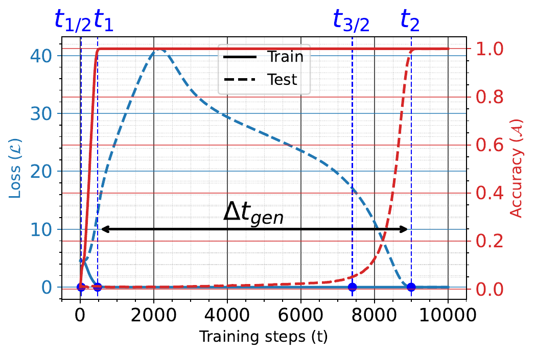
The first transition is ordinary memorization. The striking part is the long interval during which training accuracy is perfect while test accuracy remains poor, followed by generalization without any new data.

A formal definition

Let $\theta^{(t)}$ denote the parameters after $t\in\mathbb N$ optimization steps. The model optimization process can be divided into three consecutive phases when studying delayed generalization (see the figure above). The initial learning phase, $t \in [0,t_{1/2}]$, is called the confusion phase, during which both training and validation performance are poor. During the memorization phase, $t \in [t_1,t_{3/2}]$, training performance is nearly perfect while validation performance remains low. During the comprehension phase, $t \in [t_{3/2},\infty)$, validation performance improves and can eventually match training performance at step $t_2$. For a classification task such as the example above, $t_{1/2}$ can be taken as the first step at which the training accuracy $\mathcal{A}_{\text{train}}$ becomes strictly greater than $0\%$; $t_1$ as the first step at which $\mathcal{A}_{\text{train}}$ reaches $\approx1$; $t_{3/2}$ as the first step at which the test accuracy $\mathcal{A}_{\text{test}}$ becomes strictly greater than $0\%$; and $t_2$ as the first step at which $\mathcal{A}_{\text{test}}$ reaches $\approx1$.

The training of a deep-learning model by gradient descent generally, but not necessarily, goes through these phases. In the literature, training that ends in the confusion, memorization, or comprehension phase is referred to as underfitting, overfitting, or generalization, respectively.

More formally, define:

for $\mathcal B\in\{\mathcal D_{\mathrm{train}},\mathcal D_{\mathrm{test}}\}$. This is the accuracy after $t$ optimization steps. We write the two instances of Equation (3) as $\mathcal A_{\mathrm{train}}$ and $\mathcal A_{\mathrm{test}}$.

Fix a near-perfect accuracy threshold $q\in(1/p,1]$. The memorization and generalization times are

where $\inf\varnothing=\infty$. When both times are finite, the generalization delay is

Definition Choose $q$ and a minimum relative delay $\kappa>0$ before looking at the trajectory. A run exhibits grokking when

$$\begin{equation} \begin{gathered} 0<t_1<t_2<\infty, \qquad \frac{\Delta t_{\mathrm{gen}}}{t_1}\geq\kappa,\\ \mathcal A_{\mathrm{train}}(t)\geq q \quad\text{for every }t_1\leq t\leq t_2. \end{gathered} \end{equation}$$

The last condition distinguishes delayed generalization after memorization from two unrelated threshold crossings. The constant $\kappa$ gives a precise meaning to a “long” delay; suddenness is common in grokking curves, but it is not part of the definition.

Remark For the sake of simplicity, many works studying grokking characterize all training experiments that eventually generalize as grokking, thereby avoiding a debate about what could be considered a trivial number of steps.

Remark The definition above is not fully general because it assumes an ideal context in which training progresses “smoothly.” It ignores progressive sharpeningThe largest Hessian eigenvalue $\lambda_{\max}(\mathcal H^{(t)})$ increases during training, so the local loss landscape becomes progressively sharper. Cohen et al. (2021) observed it approaching the gradient-descent stability scale $2/\alpha_t$., studied by Cohen et al. (2021), and the resulting edge-of-stability regimeWhen curvature is near or beyond the nominal stability threshold $2/\alpha_t$, individual gradient-descent steps need not decrease the loss, even though the longer-run trajectory can continue to make progress.. It also ignores the slingshot mechanismThe slingshot mechanism consists of cyclic transitions between relatively stable and unstable training regimes, often accompanied by spikes in loss or parameter norm. studied by Thilak et al. (2022). The phases must therefore be adapted to the context. Lyu et al. (2023) even observed misgrokkingIn misgrokking, the model first generalizes and then, after a long training period, moves toward memorization and worse generalization—the temporal order is reversed..

From a run to a random regime

For a fixed choice $H$ of hyperparameters (e.g., learning rate, weight decay, and mini-batch size), the training split, initialization, minibatch order, and any stochastic optimizer choices make the trajectory random. Let $\omega$ denote their joint outcome under a fixed experimental protocol, and write $t_1(\omega)$, $t_2(\omega)$, $\Delta t_{\mathrm{gen}}(\omega):=t_2(\omega)-t_1(\omega)$, and $\mathcal A_{\mathrm{train}}^\omega$ for the corresponding quantities. The grokking event is

Grokking corresponds to $\mathbb P_{\mathrm{gen}}\!\left[\mathsf G_{q,\kappa}(H)\right]=1$, where $\mathbb P_{\mathrm{gen}}$ is the probability law of the random experiment. This is a statement about the full grokking event, not merely eventual test success. A finite collection of seeds can estimate its probability but cannot prove that it is one; a run stopped before $t_2$ is observed is right-censoredWe know only that the unobserved generalization time exceeds the stopping time. Treating such a run as if $t_2=\infty$ would confuse missing future observation with evidence of non-generalization., rather than evidence that $t_2=\infty$.

Although it is easy to identify grokking, it is very difficult to give a formal definition of its opposite since, in practice, we cannot optimize a model for an infinite number of steps. In many cases, we do not even have access to the true data distribution $\mathbb P_{\mathrm{data}}$ needed to properly define $\mathbb P_{\mathrm{gen}}$. Even if this distribution is available, exactly or approximately, computing $\mathbb P_{\mathrm{gen}}\!\left[\mathsf G_{q,\kappa}(H)\right]$ for a fixed choice of hyperparameters remains intractable given the complexity of the stochastic process defined by the optimization procedure, a complexity inherited in part from that of the model whose parameters are being optimized.

Faced with this challenge, we proceeded empirically in Notsawo et al. (2023). For models of the same family—that is, with the same architecture—and a given quantity of training data $r$, we train several models with different hyperparameters and initializations. When all possible input-output pairs form a finite, tractable dataset, as in addition modulo a small prime integer, $r\in[0,1]$ can instead denote the training-data fraction. We fit a function that predicts $t_2$, the generalization step, for each $r$. Then, if for a given choice of hyperparameters, initialization, and $r$, we train a model for more than the predicted $t_2(r)$ steps without generalization, we can stop training and report the outcome as confusion or memorization—that is, non-grokking—according to the observed training and validation performance. This corresponds to an empirical definition in which we use the empirical measure $\widehat{\mathbb P}_{\mathrm{gen}}$$\mathbb P_{\mathrm{gen}}$ is the ideal distribution over all runs allowed by the protocol. $\widehat{\mathbb P}_{\mathrm{gen}}$ places equal mass on the finite runs actually observed and therefore only estimates that population law. instead of $\mathbb P_{\mathrm{gen}}$.

In general, more data leads to faster grokking: $t_2(r)$ is a decreasing function of $r$, as reported by Power et al. (2022), Liu et al. (2023), Žunkovič and Ilievski (2022), and Gromov (2023). Some authors report a power law$t_2(r)=\Theta(r^{-\gamma})$ means that, up to constant factors, the generalization time scales like $r^{-\gamma}$. On logarithmic axes, this relationship appears approximately linear with slope $-\gamma$. (Žunkovič and Ilievski, 2022; Notsawo et al., 2023):

This law generally breaks at a critical value $r_c>0$Below $r_c$, the available data do not identify the target well enough for the scaling law to continue. In inverse problems, this can coincide with an information-theoretic recovery threshold.: it is valid only for $r\geq r_c$. In the toy model of Liu et al. (2023), $r_c$ can be estimated using the quality of the representations learned by the model. For sparse recovery and matrix factorization problems, for which we recently proved the existence of grokking in Notsawo et al. (2025), this limit is the minimum number of measurements below which no recovery is possible by any method whatsoever; see, for example, Rauhut (2010) for sparse recovery and Candès and Recht (2012) for matrix completion.

The three phases

This definition separates a grokking trajectory into three phases:

Taking $q=1$ for the curve above gives $\Delta t_{\mathrm{gen}}\approx8530$: the memorization phase lasts much longer than the initial fitting phase.

Liu et al. (2023) used the terms confusion, memorization, and comprehension in a phase diagram based on different hyperparameters. In this post, we also use them to refer to phases along a single training trajectory, as defined above.

It is common in the deep-learning literature to divide neural-network optimization into two phasesThe usual picture has an initial fitting phase with a small generalization gap, followed by overfitting as test error rises. Grokking requires a different temporal pattern: a prolonged memorization interval followed by improved generalization. (Shwartz-Ziv and Tishby, 2017; Nakkiran et al., 2020; Feng and Tu, 2021). However, Nakkiran et al. (2020) show that in some regimes the test error decreases again and can reach a lower value at the end of training than at the first minimum, suggesting potential training phases to exploit. Feng and Tu (2021) distinguish an initial fast-learning phase, in which the loss decreases quickly and sometimes abruptly, followed by an exploration phase, in which the training error has reached its minimum and the overall loss continues to decrease, but much more slowly and gradually. The defining ingredient of grokking lies in the memorization phase and in the transition from memorization to generalization.

Remark The definition of grokking evolved between 2024 and 2025. Initially, grokking, as observed by Power et al. (2022), corresponded to a sudden transition from a long phase of perfect memorization to generalization. Over time, however, the term has evolved to the point where, when a model generalizes late—whether abruptly or gradually—some authors refer to it as grokking. This is the case in Wang et al. (2024) and Abramov et al. (2025), who show that grokking enables Transformers to develop reasoning abilities that emerge only after extended training, whether on synthetic comparison or composition tasks or on real-world multi-hop reasoning augmented with inferred facts.

In general, this type of “reasoning” task exhibits a typical progression during training: training and test performance improve similarly from the beginning of training until the model reaches a more or less acceptable level of generalization. Then, when the model is trained for longer, a gradual increase in generalization performance is observed. We will return to this type of grokking in a future post. This seems to be the best kind of grokking we can have on “real,” non-synthetic tasks.

Accuracy is not always the right observable

Accuracy is natural for modular arithmetic, but it is only one possible observable. A smooth change in the logits can look abrupt after taking an $\operatorname{argmax}$, so loss curves should be shown as well. In regression, signal recovery, or matrix completion, the same definition can use predeclared error tolerances instead of accuracy thresholds.

In contexts where accuracy is not directly available, such as regression, one can use the value $\mathcal L$ of the loss function directly, so that “$\mathcal A\approx1.0$” becomes “$\mathcal L\approx0$.” Alternatively, following Liu et al. (2023), one can define accuracy as the empirical fraction of points whose prediction error is smaller than a chosen tolerance $\epsilon\geq0$:

where $\ell(z)$ is the value of the loss function on the sample $z$. Here the hat and indicator$\widehat{\mathbb E}$ and $\widehat{\mathbb P}$ average over the finite dataset, while $\mathbf 1\{\ell(z)\le\epsilon\}$ equals $1$ when the tolerance is met and $0$ otherwise. Their average is therefore the fraction of successful samples. turn a continuous error into an empirical accuracy.

It should be noted that the transition in $\mathcal L(t)$ is generally not as sharp as the transition in $\mathcal A(t)$, and it is possible to observe a transition in $\mathcal A(t)$ without observing one in $\mathcal L(t)$, as shown by Kumar et al. (2023). It is preferable to study grokking using loss rather than accuracy: loss reflects the training dynamics, whereas accuracy is discontinuous and can exhibit apparent transitions without any internal change in the model. As Kumar et al. (2023) point out in the context of grokking, hard-threshold measures of performance such as accuracy can be extremely misleading; continuously optimized measures such as loss should be studied instead (Schaeffer et al., 2024).

The observable must match the scientific question. In sparse recovery, measurement residual and recovery error answer different questionsA small residual means the estimate matches the observed measurements. A small recovery error means it is close to the unknown latent signal. With insufficient or ambiguous measurements, the former can be tiny while the latter remains large.. Confusing the two can produce what we call grokking without understanding in the next post.

What to report

A grokking experiment should report:

• the task, split, model, optimizer, and regularization;
• the observable and the chosen values of $q$ and $\kappa$;
• the training and test curves, together with $t_1$, $t_2$, and $\Delta t_{\mathrm{gen}}$ across seeds.

With these choices fixed, grokking is no longer just the shape of one attractive curve. It is a measurable event: rapid memorization, a non-trivial delay, and eventual generalization.

References

• Alethea Power, Yuri Burda, Harri Edwards, Igor Babuschkin, and Vedant Misra, “Grokking: Generalization Beyond Overfitting on Small Algorithmic Datasets”, 2022.
• Jeremy M. Cohen, Simran Kaur, Yuanzhi Li, J. Zico Kolter, and Ameet S. Talwalkar, “Gradient Descent on Neural Networks Typically Occurs at the Edge of Stability”, ICLR 2021.
• Vimal Thilak, Etai Littwin, Shuangfei Zhai, Omid Saremi, Roni Paiss, and Joshua Susskind, “The Slingshot Mechanism: An Empirical Study of Adaptive Optimizers and the Grokking Phenomenon”, 2022.
• Kaifeng Lyu, Jikai Jin, Zhiyuan Li, Simon S. Du, Jason D. Lee, and Wei Hu, “Dichotomy of Early and Late Phase Implicit Biases Can Provably Induce Grokking”, 2023.
• Pascal Jr Tikeng Notsawo, Hattie Zhou, Mohammad Pezeshki, Irina Rish, and Guillaume Dumas, “Predicting Grokking Long Before It Happens: A Look into the Loss Landscape of Models Which Grok”, 2023.
• Ziming Liu, Ziqian Zhong, and Max Tegmark, “Grokking as Compression: A Nonlinear Complexity Perspective”, 2023.
• Bojan Žunkovič and Enej Ilievski, “Grokking Phase Transitions in Learning Local Rules with Gradient Descent”, 2022.
• Andrey Gromov, “Grokking Modular Arithmetic”, 2023.
• Pascal Jr Tikeng Notsawo, Guillaume Dumas, and Guillaume Rabusseau, “Grokking Beyond the Euclidean Norm of Model Parameters”, 2025.
• Holger Rauhut, “Compressive Sensing and Structured Random Matrices”, in Theoretical Foundations and Numerical Methods for Sparse Recovery, 2010.
• Emmanuel Candès and Benjamin Recht, “Exact Matrix Completion via Convex Optimization,” Communications of the ACM 55(6):111–119, 2012.
• Ravid Shwartz-Ziv and Naftali Tishby, “Opening the Black Box of Deep Neural Networks via Information”, 2017.
• Preetum Nakkiran, Gal Kaplun, Yamini Bansal, Tristan Yang, Boaz Barak, and Ilya Sutskever, “Deep Double Descent: Where Bigger Models and More Data Hurt”, ICLR 2020.
• Yu Feng and Yuhai Tu, “The Inverse Variance–Flatness Relation in Stochastic Gradient Descent Is Critical for Finding Flat Minima”, Proceedings of the National Academy of Sciences 118(9):e2015617118, 2021.
• Boshi Wang, Xiang Yue, Yu Su, and Huan Sun, “Grokked Transformers Are Implicit Reasoners: A Mechanistic Journey to the Edge of Generalization”, 2024.
• Roman Abramov, Felix Steinbauer, and Gjergji Kasneci, “Grokking in the Wild: Data Augmentation for Real-World Multi-Hop Reasoning with Transformers”, 2025.
• Ziming Liu, Eric J. Michaud, and Max Tegmark, “Omnigrok: Grokking Beyond Algorithmic Data”, ICLR 2023.
• Tanishq Kumar, Blake Bordelon, Samuel J. Gershman, and Cengiz Pehlevan, “Grokking as the Transition from Lazy to Rich Training Dynamics”, 2023.
• Rylan Schaeffer, Brando Miranda, and Sanmi Koyejo, “Are Emergent Abilities of Large Language Models a Mirage?” Advances in Neural Information Processing Systems 36, 2024.

@misc{tikengnotsawo2025whatisgrokking,
  author = {Tikeng Notsawo, Pascal Jr.},
  title = {{What Is Grokking? A Formal Definition}},
  year = {2025},
  month = may,
  url = {https://tikquuss.github.io/blog/what-is-grokking/},
  note = {Blog post}
}