Generating Random Variables and Stochastic Processes, Generative Flow Networks (GFlowNets)
2 minute read
Published:
Note: It's better to read all the updates below before clicking on any link.
Practical tutorial
Here here is the practical tutorial (theory & code) I wrote in Winter 2022 about GflowNets [1], MCMC, Metropolis-Hasting, Gibbs sampling, Metropolis-adjusted Langevin, Inverse Transform Sampling, Acceptance-Rejection Method and Important Sampling. I received a lot of positive feedback on this tutorial, which has been the starting point for many in their learning of GflowNets.
More resources
To go in depth with GflowNets : GflowNets foundations paper [2] or Trajectory Balance paper [3] (very pedagogical paper).
For Variational Bayes, I recomment the paper A practical tutorial on Variational Bayes [4]
See also MCMC and Bayesian Modeling, 2017, Martin Haugh, Columbia University
Update : I met Pierre L’Ecuyer
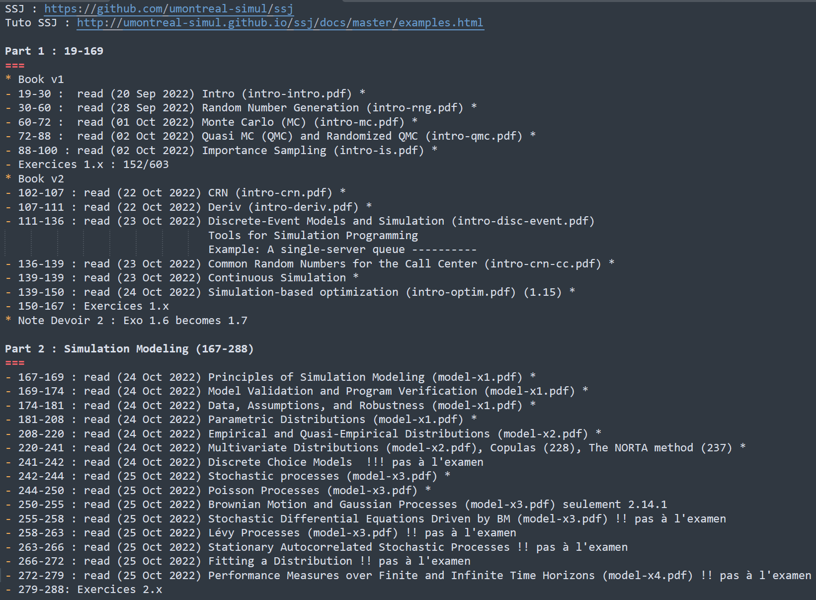
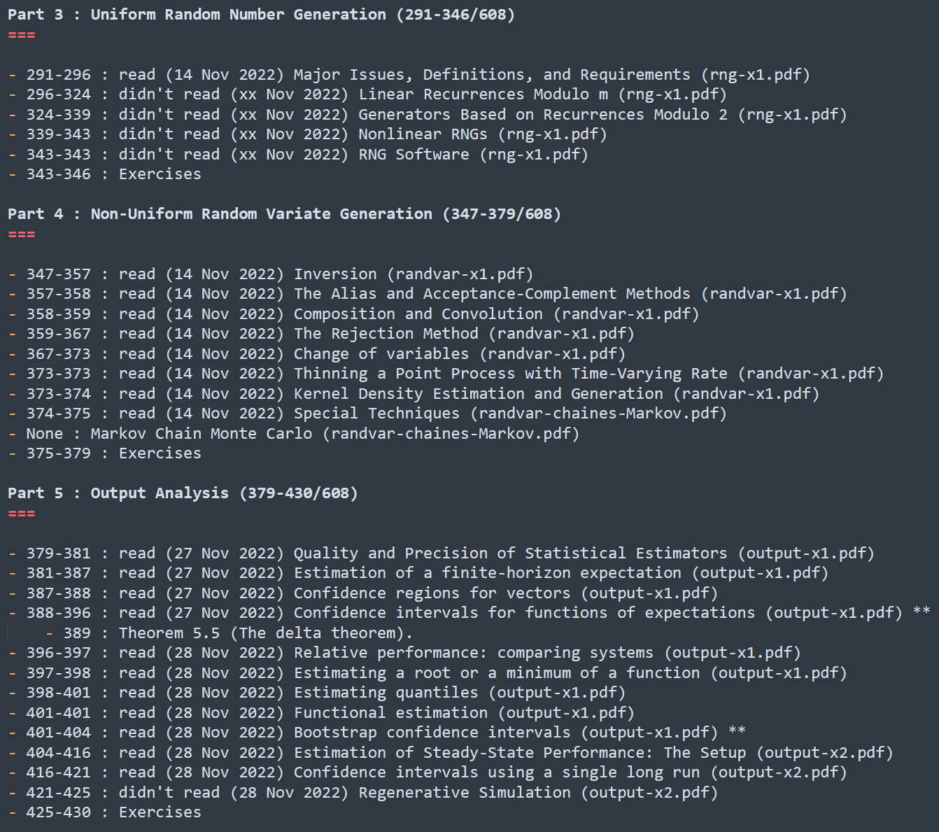
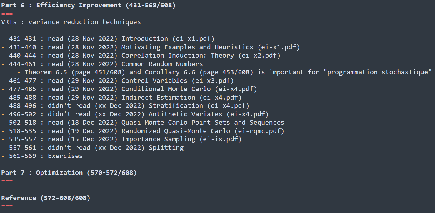
In Fall 2022, wanting to update my level in probability and statistics, I took "IFT6561 : Stochastic Simulation", taught at the Université de Montréal by the eminent Pierre L'Écuyer. This course is clearly a masterclass. It's very theoretical and very practical at the same time. Pierre L'Écuyer is the 2nd best teacher I've known in my life so far. I was very close to switching to another field, since he was planning to take me on as a student; but unfortunately I was already being supervised. His book, "Stochastic Simulation and Monte Carlo Methods", a masterclass, is not yet public. But if you ask for access he will send it to you. Here are the book's headlines, captured from my reading plan (Click on each image to zoom in - I've noticed that it only works locally, so just open the image in the new tab).
×
Note: I mention this section because I'm supposed to add a section on Gibbs sampling, Metropolis-adjusted Langevin and Important Sampling to my tutorial by now, from the book of Pierre. I'll find the time to do it so that the tutorial can be complete.
Grokking refers to a delayed generalization following overfitting when optimizing artificial neural networks with gradient-based methods. We show that the dynamic of grokking goes beyond the $\ell_2$ norm, that is: If there exists a model with a property $P$ (e.g., sparse or low-rank weights) that fits the data, then GD with a small (explicit or implicit) regularization of $P$ (e.g., $\ell_1$ or nuclear norm regularization) will also result in grokking, provided the number of training samples is large enough. Moreover, the $\ell_2$ norm of the parameters is no longer guaranteed to decrease with generalization when it is not the property sought.
Let’s suppose we’re training a model parameterized by $\theta$, and let’s denote by $\theta_t$ the parameter $\theta$ at step $t$ given by the optimization algorithm of our choice. In machine learning, it is often helpful to be able to decompose the error $E(\theta)$ as $B^2(\theta)+V(\theta)+N(\theta)$, where $B$ represents the bias, $V$ the variance, and $N$ the noise (irreducible error). In most cases, the decomposition is performed on an optimal solution $\theta^*$ (for instance, $\lim_{t \rightarrow \infty} \theta_t$, or its early stopping version), for example, in order to understand how the bias and variance change with the complexity of the function implementing $\theta$, the size of this function, etc. This has helped explain phenomena such as model-wise double descent. On the other hand, it can also be interesting to visualize how $B(\theta_t)$ and $V(\theta_t)$ evolve with $t$ (which can help explain phenomena like epoch-wise double descent): that’s what we’ll be doing in this blog post.