A common practice in deep learning is to stop training a model as soon as a sign of overfitting is observed, or when the model’s generalization capabilities have not improved over a long training period (early stopping). The limits of this practice are now well-known today, since (i) a model’s performance can improve, deteriorate and then improve again during training (epoch-wise double descent) (ii) a model can generalize several steps after severe overfitting (grokking). Epoch-wise double descent and grokking open the way to new studies concerning the structure of the minimum found by Stochastic Gradient Descent (SGD), and how networks behave in the neighbourhood of SGD training convergence. These phenomena also lead us to rethink our knowledge about the relationship between the model size, data size, initialization, hyperparameters and generalization of neural networks. Beyond just rethinking this relationship, there appears to be a need to be able to identify measures that are easy and cheaper to obtain and that are strongly correlated with generalization since phenomena such as multiple descents can occur at model sizes that are difficult to experiment with, just as grokking often requires models to be trained for a very large number of epochs, making it difficult to construct a phase diagram of generalization covering all the hyperparameters. With these issues in mind, we’ve been looking at grokking recently [1]. This blog post summarizes some of the observations we’ve made.

Grokking

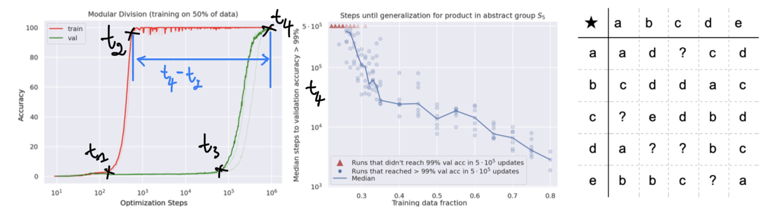
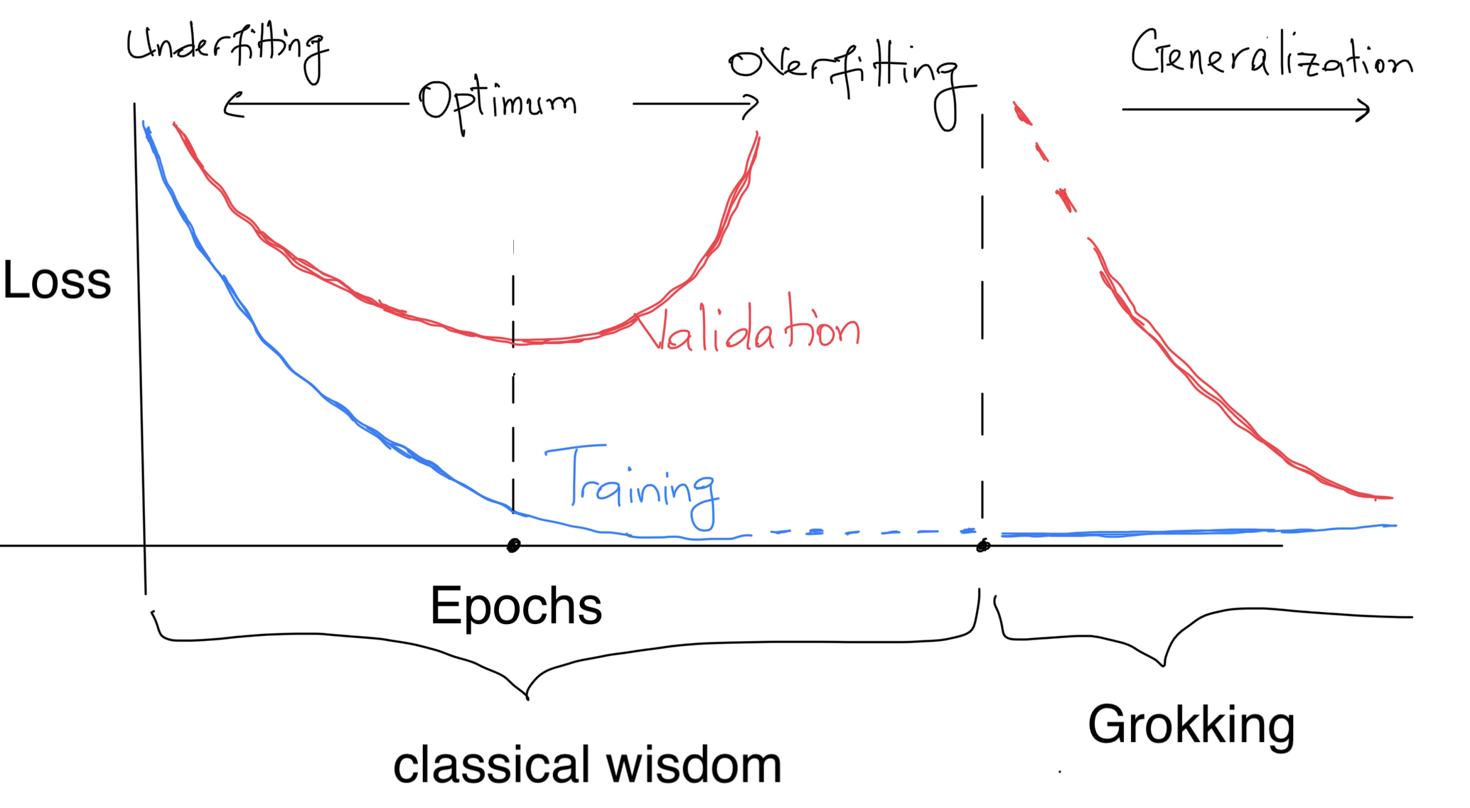
We will distinguish from the above figure four learning phases :

• Confusion : $t \in [0, t_1]$
• Memorization : $t \in [t_2, t_3]$
• Comprehension : $t \in [t_3, \infty]$
• Generalization : $\mathbb{P}[t_4 < \infty] = 1$ (i.e. when $t_4 < \infty$ almost surely)
  The measure $\mathbb{P}$ captures randomness in initialization, choice of training and validation points, noise in optimization…
  Grokking $\approx$ generalization with $t_4 \gg t_2$.

The order we establish between these phases is only valid within the specific framework of grokking observed on this algorithmic data. On other tasks, these phases can be in any order, overlapping or repeating themselves… In practice, when the model converges (or its training is stopped) during a phase of confusion, we term this underfitting. When it does so during memorization, we refer to it as overfitting.

Grokking is a generalization that comes very late after overfitting/memorization ($t_4 \gg t_2$). “Late” is relative here, as everyone can choose his own threshold, and as soon as $t_4 - t_2$ is above this threshold, he considers the phenomenon to be grokking.

Spectral Signature of the loss is correlated to generalization

When we reproduced the code from the original paper [2], we found that the model sometimes needs to be trained for more than 100k epochs to observe any sign of generalization when the training data size becomes smaller and smaller. This raises the question of whether or not grokking can be predicted. We answer this question in the affirmative by showing that the spectral signature of the learning curves of a transformer network trained on arithmetic data (“algorithmic datasets” in previous work) in early epochs can serve as a proxy to the upcoming grokking phenomenon. The proposed spectral signature is derived by applying the Fourier transform to quantify the amplitude of low-frequency components in the training loss curve.

This spectral signature is based on Hjorth’s parameters (activity, mobility and complexity). We used activity, and highlight below how it relates to mobility and complexity. Let $L(t)$ the loss at $\theta(t)$ (the parameter update at time $t$ given the optimization algorithm of choice), $G(t) = \nabla_{\theta} L(t)$ the gradient of the loss function at $\theta(t)$ and $\mathcal{H}(t) = \nabla^2_{\theta} L(t)$ the Hessian matrix of the loss at $\theta(t)$. Let ${ \lambda_i(t) }$ be the spectrum of $H(t)$, and ${ V_i(t) }$ the associated eigenvectors. Let also $\mathcal{F}(L)$ denote the Fourier transform of $L(t)$ and $m_n(L) = \int \omega^n | \mathcal{F}(L)(\omega) |^2 d \omega$, the $n^{th}$ moment of $\mathcal{F}^2 (L)$, with $|\mathcal{F}(L)(\omega)|^2$ the energy spectral density present in the pulse $\omega$.

From the gradient flow equation $\dot{\theta} = - G(t)$, it holds that $\dot{L} \approx - G(t)^T G(t)$ and $\ddot{L} \approx 2 G(t)^T H(t) G(t) = 2 \sum_{i} \lambda_i(t) \langle G(t), V_i(t) \rangle^2$. This clarifies why the evolution of $L$ over time depends on the norm of the gradient, and how fast it changes depending on the curvature of its landscape.

• The Hjorth activity represents the signal power, the surface of the power spectrum in the frequency domain. It is given by $m_0(L)$, which is equal to $\int L^2 (t) dt$ by the parseval’s theorem.
• The Hjorth mobility is the mean frequency or the proportion of standard deviation of the power spectrum and is given by $\sqrt{m_2 (L) / m_0(L)}$ with $m_2(L) = \int | \omega \mathcal{F}(L)(\omega)|^2 d \omega$. It is easy to see that $m_2(L) = \int \dot{L}^2 (t) dt \approx m_0 (\dot{L})$, which is activity of the gradient norm $| G(t) |^2$.
• The Hjorth complexity, which indicates how the shape of a signal is similar to a pure sine wave, is given by $\sqrt{m_4 (L) / m_2(L)}$ with $m_4(L) = \int | \omega^2 \mathcal{F}(L)(\omega)|^2 d \omega$. We also have $m_4(L) = \int \ddot{L}^2 (t) dt \approx m_0 (\ddot{L})$, which is the activity of the hessian spectrum.

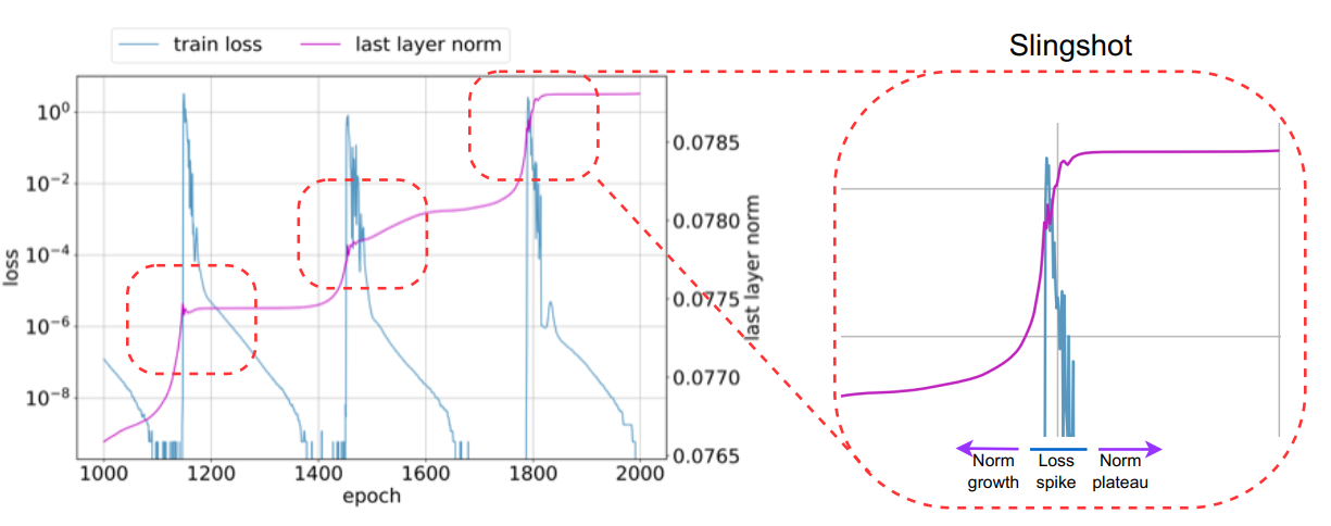
This figure shows a similarity between the oscillation in the training loss in the early phases of training and the validation accuracy, suggesting that the spectral signature can serve as a proxy for the upcoming grokking phenomenon. This observation is related to the slingshot effect [3], which was observed to generally come in tandem with grokking, that is grokking almost exclusively happens at the onset of slingshots, and is absent without it.

This spectral signature can be classified as an optimization-based generalization measure, which is known to be highly predictive of generalization [4] (other optimization-based measures include the speed of the optimization, stability, etc). In fact, the results of [4] suggest that the difficulty of optimization during the initial phase of the optimization benefits the final generalization, but the evolution of the loss when it reaches a certain value is not correlated to the generalization of the final solution. The advantage of optimization-based generalization measurements is that they are generally only made on the training dataset and only require the model to be trained for a small number of epochs, compared with measurements such as sharpness-based measures which, as their name suggests, require the to train the moment until convergence. Importantly, such a measure is not an explicit capacity measure so either positive or negative correlation with generalization could potentially be informative.

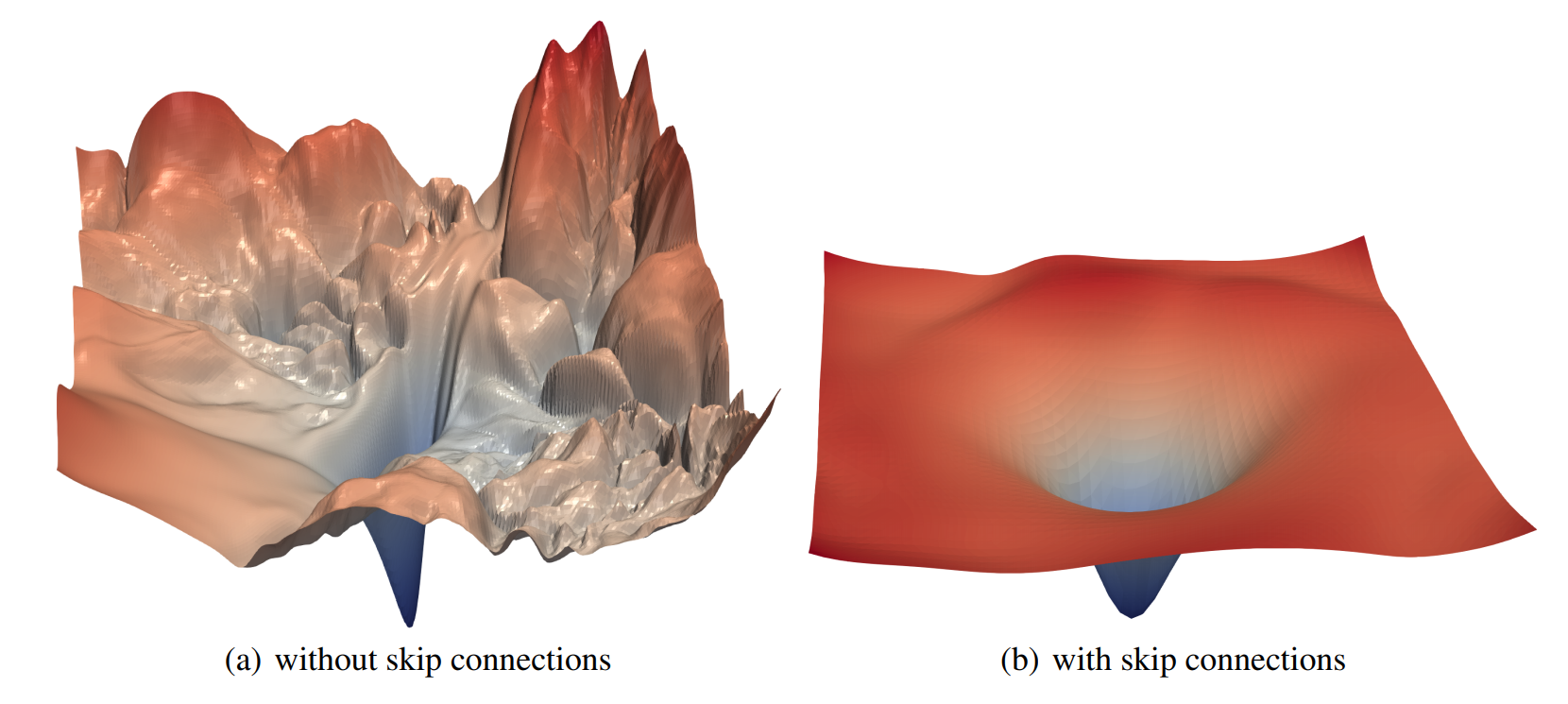
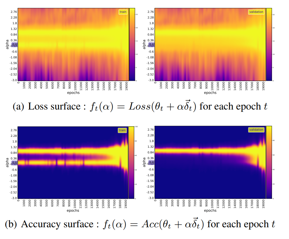
Grokking is a result of a (random) walk in a valley of local solution

A strong correlation between the frequency of oscillations in the loss and the generalization performance of the model supports the fact that the learning behaviour of the model is tightly coupled with the training loss, but does not give enough information about the behaviour of the model weights before and after grokking. Does the model, before grokking, oscillate around a local minimum, cross a very flat region, or circumvent a large obstacle? By observing the landscape of the model, we conclude that the model crosses a perturbed valley of bad/local solutions before grokking. When the iterates fall in the valley, we are at the minimum for the training objective, so that the model can memorize the training data, and it achieves grokking when it successfully breaks free from the basin of attraction of such solutions.

We also observe that :

• the Hessian of the grokking loss function is characterized by larger condition numbers, leading to a slower convergence of gradient descent.
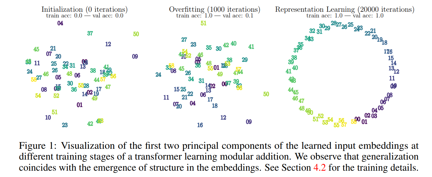
• more than $98\%$ of the total variance in the parameter space occurs in the first $2$ PCA modes much smaller than the total number of weights, suggesting that the optimization dynamics are embedded in a low-dimensional space.
• the model remains in a lazy training regime most of the time, as the measure of cosine distance between the model weights from one training step to the next remains almost constant, except at the slingshot location.

These observations are not isolated facts. Some works (eg [5]) hypothesize that SGD finds good solutions only if they are surrounded by a relatively large volume of solutions that are nearly as good, as we saw above with grokking optimum that is surrounded by many local minima along the principal directions of curvature. [5]’s work focuses on showing that, under realistic hypotheses, SGD performs implicit regularization or tends to find solutions that possess some particular structural property that we already know to be connected to generalization, like widder minima, that are less difficult to reach by SGD than sharper one as they have a large basin of attraction.

These are also link to the linear form of mode connectivity, a phenomenon where the minima found by two networks are connected by a path of nonincreasing error. Beren’s blog post makes this point (without explicitly mentioning the word) clear as follows. For an underparametrized network, the optimal set—comprising all parameter values that lead to a training loss of $0$ on the dataset—is empty. As the representational capacity increases, we reach the threshold of perfectly parametrized models, where there exists a single optimal point (though reaching it is a random event). By continuing to add parameters and enhance the representational capacity of the network, we obtain overparametrized networks, revealing an infinite number of solutions resulting in 0 training loss. As the network becomes more and more overparametrized, we observe scattered points and eventually witness the formation of ‘islands’ of optimality. Although there might be an infinite number of such islands and potentially infinite ‘channels’ connecting them, which may represent redundant or nuisance parameter dimensions, it is crucial to note that the volume of the optimal set remains incredibly small compared to the non-optimal set. At the begening of training, the network moves towards a nearby island. Unfortunately, this island corresponds to a poor solution in terms of validation loss. As SGD explores the small region around this island, it gets trapped, unable to escape due to the surrounding vast suboptimality. The gradient noise prevents it from tunnelling across the suboptimality to reach other islands. Consequently, the network remains stuck, unable to grok or achieve good generalization; it is stuck in a state of overfitting indefinitely. As the number of parameters increases, the volume of the optimal set relative to the total parameter space expands. The islands of optimality become closer and eventually merge, creating extensive connected optimal surfaces or manifolds in the parameter space. With a sufficiently large number of parameters, even tending to infinity, the optimal set effectively covers the entire parameter space, lying infinitesimally close to all points. This expansive coverage of the parameter space allows the network to generalize better, escaping the overfitting issue experienced with insufficient parameterization.

Some related works

Why is it important to study such phenomena?

Understanding all this behaviour and how they affect the predictive performance of neural networks (for example, at scale or out-of-distribution, in continual learning settings…) is relevant to safety or may have potential safety consequences. In fact, a central problem is that we may need to be certain of the safety of a model before we scale it to a capability level beyond which we cannot control it [8], or transfer its knowledge from one task to another. This is particularly concerning because the out-of-distribution generalization behaviour of deep learning models is known to be challenging to control or foresee.

References

[1] Predicting Grokking Long Before it Happens: A look into the loss landscape of models which grok

[2] Grokking: Generalization Beyond Overfitting on Small Algorithmic Datasets

[3] The Slingshot Mechanism: An Empirical Study of Adaptive Optimizers and the Grokking Phenomenon

[4] Fantastic Generalization Measures and Where to Find Them

[5] Computing Nonvacuous Generalization Bounds for Deep (Stochastic) Neural Networks with Many More Parameters than Training Data

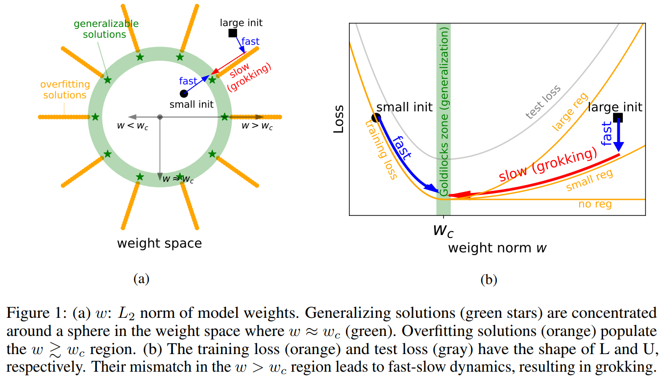
[6] Omnigrok: Grokking Beyond Algorithmic Data

[7] Towards Understanding Grokking: An Effective Theory of Representation Learning

[8] Unifying Grokking and Double Descent

Aren’t headings cool?